AUTOMATIC EXTRACTION OF DTM FROM LOW RESOLUTION DSM BY
TWO-STEPS SEMI-GLOBAL FILTERING
Yanfeng Zhang a, Yongjun Zhang a,*, Yi Zhang a, Xin Li a
a School of Remote Sensing and Information Engineering, Wuhan University, Wuhan 430079, China- [email protected], [email protected], [email protected], [email protected]
Commission III, WG III/2
KEY WORDS: DTM, DSM, Slope map, Semi-Global Filtering, Segmentation, Classification
ABSTRACT:
Automatically extracting DTM from DSM or LiDAR data by distinguishing non-ground points from ground points is an important issue. Many algorithms for this issue are developed, however, most of them are targeted at processing dense LiDAR data, and lack the ability of getting DTM from low resolution DSM. This is caused by the decrease of distinction on elevation variation between steep terrains and surface objects. In this paper, a method called two-steps semi-global filtering (TSGF) is proposed to extract DTM from low resolution DSM. Firstly, the DSM slope map is calculated and smoothed by SGF (semi-global filtering), which is then binarized and used as the mask of flat terrains. Secondly, the DSM is segmented with the restriction of the flat terrains mask. Lastly, each segment is filtered with semi-global algorithm in order to remove non-ground points, which will produce the final DTM. The first SGF is based on global distribution characteristic of large slope, which distinguishes steep terrains and flat terrains. The second SGF is used to filter non-ground points on DSM within flat terrain segments. Therefore, by two steps SGF non-ground points are removed robustly, while shape of steep terrains is kept. Experiments on DSM generated by ZY3 imagery with resolution of 10-30m demonstrate the effectiveness of the proposed method.
1. INTRODUCTION
DTM (Digital Terrain Model) is an important surveying product, which can be used in many applications such as terrain analysis (White and Wang, 2003; Martha et al., 2010; Zhan et al., 2015) and generation of DOM (Digital Ortho Map) or TDOM (True Ortho Map) (Habib et al., 2007), etc. DTM contains only terrain information while elevation dataset like LiDAR data or DSM (Digital Surface Model) generated by image matching consists of both terrains and surface objects which are known as ground points and non-ground points, respectively. Therefore, in order to get DTM, non-ground points need to be identified and removed from LiDAR data or DSM, such process is called as filtering (Vosselman and Sithole, 2004). Advancement of LiDAR (Light Detection and Ranging) techniques impels abundant of valuable research achievements for extraction of high resolution DTM from LiDAR data in urban area, such as mathematical morphological methods (Zhang et al., 2003; Chen et al., 2007; Pingel et al., 2013), interpolation based methods (Kraus and Pfeifer, 1998), TIN based methods (Axelsson, 2000), slope based methods (Vosselman, 2000; Sithole, 2001), and scan line based methods (Meng et al., 2009), etc. LiDAR dataset usually has a density of at least one point per square meter, thus topographic relief prominently differs from non-ground points in perspective of elevation variation (Figure 1). Therefore, filtering algorithms hold an assumption that elevation variation of topographic relief is smooth while that of non-ground points is abrupt. As a result, most of filtering methods perform well in flat terrains but they are prone to fail in steep terrains, where there is almost no difference between topographic relief and non-ground points. Though DTM from LiDAR is of great significance, especially in urban areas, low resolution DTM can be useful in a coarser and larger scale. Low resolution DTM is usually generated by
filtering DSM, which is produced by dense matching of satellite imagery (Gruen, 2012). However, in contrast of the generation of DSM, the automatic extraction of DTM from DSM has been scarcely studied, and DTM is usually produced by manual editing.
It seems possible that methods for LiDAR filtering can be used for DSM. However, characteristic of DSM does not fit the assumption of such methods. When point cloud density is low, or with a low resolution, slope caused by non-ground points will decrease evidently, which will make the elevation variation caused by steep terrains and non-ground points unable to distinguish (Figure 1). Therefore, it’s conflict to keep the shape of steep terrains and filter the non-ground points at the same time. Recently a method proposed by Sreedhar et al. (Sreedhar et al., 2015) is aimed at solving this problem by densifying DSM data, and making it similar to LiDAR data, thus mathematical morphological methods can be used to handle this problem. However, multi-source DSM data is needed, which leads to the limitation of the practicability.
Though steep terrains and non-ground points cannot be distinguished by local slope, two characteristics of low resolution DSM make it possible to extract DTM automatically: Firstly, large slope is very dense at steep mountainous terrains, and relatively sparse at flat terrains with non-ground points, which means steep terrains and flat terrains (with non-ground points) have different non-local terrain characteristic. Secondly, it’s almost unnecessary to filter steep mountainous terrains of low resolution DSM, while it’s the flat terrains with large ground objects that is the key areas for filtering. Thus, the objective of this paper is to recognize and filter the flat terrain areas of DSM while keep the steep terrains from damaged. ISPRS Annals of the Photogrammetry, Remote Sensing and Spatial Information Sciences, Volume III-3, 2016
(a) (b)
(c) (d)
Figure 1. Comparison of dense LiDAR data and low resolution DSM. (a) LiDAR data with 0.5m GSD supplied by ISPRS; (b) DSM with 10m GSD interpolated with the LiDAR data; (c) Elevation profile of LiDAR data; (d) Elevation profile of DSM. It is demonstrated by (c) and (d) that elevation variation or local slope caused by non-ground points is abrupt in LiDAR data and smooth in DSM, which makes elevation variation of non-ground points in DSM indistinguishable from that caused by topographic relief.
(a) (b)
Figure 2. (a) Low resolution DSM; (b) Slope map of (a). This figure shows that slope of buildings and steep mountainous terrains tends to be large. Since buildings scattering in flat terrain areas are relatively sparse, thus, density of large slope at flat areas is relatively small, while that of large slope at mountainous terrains is large. Therefore, the above overall pattern can be used in non-local filtering to distinguish flat terrains from steep mountainous terrains.
Therefore, extracting of DTM can be divided into two steps: 1) Find flat terrains on DSM. Since there are little non-ground points in steep mountainous areas, we can first exclude this part of data in order to keep mountainous terrains. The non-local filtering of slope map can be used to increase the distinction between steep mountainous terrains and flat terrains (Figure 2). 2) Remove non-ground points on flat terrains by filtering of DSM. Filtering of both slope map and DSM can be modelled as a labelling problem in which the labels correspond to slope levels and elevation levels, respectively. Take slope map filtering as an example, we’ll first introduce the energy function for filtering in consideration of the non-local terrain characteristic.Slope map is the 2-D image of slope data at every point on DSM. Filtering of slope map is to assign new slope value to each point, which should be as close to as the original image, and as smooth as the neighbourhood points. Therefore, energy function for this issue can be constructed as follow:
( ) ( ) ( ) ( , ) ( ) neighbourhood points after filtering. The optimization of function (1) is the minimization of the whole filed energyE(s), by assign proper slope sp to every pointp. In addition, in order to keep steep terrains, piecewise smooth rather than pixelwise smooth should be used here.
2-D energy minimization with piecewise smooth is a NP hard problem and to solve it two kinds of methods are used: 1) Global optimization using MRF-MAP, such as simulated annealing (Kirkpatrick et al., 1983), ICM (Besag, 1986), graph cut (Boykov and Kolmogorov, 2004), belief propagation (Sun et al., 2003), etc. Algorithms of this category are easily trapped into local optimization or too complicated and inefficient. 2) The other kind of methods is based on simplified energy function model, i.e. firstly, the 2d problem is simplified as 1d problem, then solved by dynamic programming, which easily cause strip problem. Hirschmüller proposed the semi-global optimization method (Hirschmüller, 2008), which modified the dynamic programming method and got good results in dense matching. And it will be used in this paper to take the overall terrain characteristic in consideration.
Based on the above analysis, a filtering method called two-steps semi-global filtering (TSGF) for the generation of DTM from low resolution DSM is proposed. Firstly, the slope map of DSM is calculated and smoothed by semi-global filtering, which is then binarized and used as mask of flat terrain areas. Secondly, DSM of flat terrain areas is segmented with the restriction of flat terrain mask. Lastly, each segment is filtered with semi-global algorithm in order to remove surface objects, which will produce the final DTM. The proposed method is similar to the semi-global filtering recently proposed by Hu et al. (Hu et al., 2015). However, a locally calculated balance coefficient is added in the smooth term Esmooth( )s of energy function proposed by Hu, which makes the energy function rely on local slope heavily, thus it’s impropriate to use in DSM filtering. Contribution of this paper includes two aspects: firstly, characteristic of low resolution DSM is analyzed, and non-local method used to detect steep mountainous terrains and flat terrains before filtering is proposed. Secondly, non-local filtering with segment constraint removes non-ground points and keeps terrains at the same time.
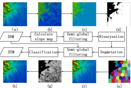
2. TWO-STEPS SEMI-GLOBAL FILTERING Since non-ground points on low resolution DSM are mainly distributed in flat terrain areas, DTM can be produced by first detecting flat terrain areas, then filtering these areas to remove non-ground points. Therefore, the proposed method contains two steps: first detecting flat terrain areas, second filtering the detected areas. Flowchart of the proposed method shows in Figure 3. Slope of every point on DSM is firstly computed, and then slope map is processed by semi-global filtering, which could smooth the slope of flat terrains at a low level and keep that of steep mountainous terrains at a relative large level. Afterwards, the filtered slope map is binarized as the mask of flat terrains. Flat terrain mask is then segmented, and semi-global filtering is used to process on each DSM segments, which will decrease the elevation of non-ground points at flat ISPRS Annals of the Photogrammetry, Remote Sensing and Spatial Information Sciences, Volume III-3, 2016
terrains, and get a classification surface, which will be used to classify ground points from non-ground points. DTM is finally generated by the interpolation of ground points.
Figure 3. Flowchart of TSGF. (a) Low resolution DSM; (b) Slope map of (a); (c) Slope map filtered by the first SGF; (d) Flat terrain mask; (e) Segmentation of flat terrain mask; (f) Classification surface generated by the second SGF; (g) Classification results in which non-ground points are labelled in white colour; (h) DTM.
2.1 Semi-Global Filtering of Slope Map
Slope is one of the most important DSM characteristics, which can be used to distinguish steep terrains from flat terrains. Two methods are usually used to calculate slope, the first one is percentage method, and the other one is degree method, which is used in this paper (Equation 2).
S
parctan(
H
p)
GSD
(2)As mentioned in the introduction, large slope value is densely distributed in mountainous terrains, while relatively sparsely distributed in flat terrains. Therefore, non-local filtering can be used to strengthen the terrain discrimination for future terrain detection. Semi-global optimization (Hirschmüller, 2008) is used here for this purpose.
Semi-global optimization is originally used in dense matching, the algorithm is first aggregating matching cost for each point from at least 8 directions independently. The aggregating function is given by 1-D energy function with piecewise smooth constraint. Then optimal disparity of each point is got by the principle of WTA (winner takes all). The original algorithm is modified in this paper as semi-global filtering by replacing matching cost with filtering cost designed for the DSM filtering problem.
Energy function of semi-global filtering for slope map is:
1 2 term represents Esmooth( )s in correspondence with Equation (1).
Specifically, srepresents slope,
P
1andP
2 are constants, whichare the penalty for slope change.
The aggregated cost of slopes in r direction of every point p is be implemented as absolute of slope difference; the second term is the minimization of 4 candidate costs based on the previous point in direction r. min (k L p r kr , ) represents the optimal cost of previous point of p in direction r. Subtracting of this term will prevent '( , )
r
L p s from increasing infinitely and not affect slope selection of point
p
, since the final value of s will not be affected by this term.Cost should be aggregated in at least 8 directions independently and then summed up as the final energy E (p, s): degree, and the discretized slope map has 90 levels. Though the process of discretization will lost precision, it has little effect on the result of future flat areas detection.
2.2 Recognition and Segmentation of Flat Terrain
After the semi-global filtering of slope map, the large slope caused by non-ground points in flat terrain areas is smoothed, while that caused by steep mountainous terrains is kept. Thus binary segmentation can be used here to generate a mask of flat terrains. Threshold used in this paper is 5 degree. However, since there are inevitably errors during binarization, thus flat terrain mask cannot be used to classify the DSM directly, which is used as prior information as an indication of the possible existing non-ground points.
Binarization will generate small patches in the mask. A simple region growing based segmentation method is used to remove these patches, which is to keep the labels of 4-connected points within one segment from varying. The points of all segments below a certain size will be identified as invalid patches, of which mask labels will be reversed. Figure 4(b) shows the effectiveness of this method.
After detection of flat terrain areas, segmentation is employed to generate processing unit of DSM filtering. Two purposes are considered to use segmentation here. Firstly, flat terrain areas ISPRS Annals of the Photogrammetry, Remote Sensing and Spatial Information Sciences, Volume III-3, 2016
that are not connected with each other have different elevation range, thus they should be processed separately, otherwise they will affect each other and lead to bad results. Secondly, elevation variation will also be quite large if the area of connected flat terrains is very large, which is bad for non-local filtering as well. Segmentation algorithm used here is superpixel method (Achanta et al., 2012), which could be replaced with other over-segmentation methods. After segmentation, flat terrain mask is divided as several segments and within each segment semi-global filtering of DSM will be implemented independently.
(a) (b) Figure 4. Removal of small patches.
2.3 Semi-Global Filtering of DSM with segment constraint DSM filtering within each segment has 3 steps: firstly, elevation of the segment is discretized and a noise removal process is done by simple histogram statistics method afterwards. Secondly, balance coefficient of every point in the segment is calculated. Lastly, DSM is processed by semi-global filter with the balance coefficient.
Discretization method used on elevation is 1) Set step number N for the processed segment, all segments will have the same number 2) Extract the maximum and minimum elevation in each segment, which will get the elevation range; 3) Divide the elevation range by step number, which will get elevation step
stepHei
i.stepHeii (maxHeiiminHeii) /N (7) In Equation (7), maxHeiiand minHeii represent the largest and smallest elevation in segment
S i
( )
. It means that both elevation step and overall elevation range for each segment will be different.Noise removal based on histogram is to first compute elevation frequency in each elevation step, and then remove elevations with frequency lower than a given threshold. After noise removal, discretization of elevation should be calculated again by Equation (7).
Equation (8) shows how to calculate the balance coefficient:
( )
H is the elevation at point
p
. The balance coefficient makes the optimal elevation selection associated with original elevation.q S i . With the balance coefficient, small elevation will be kept while large ones will be smoothed, which corresponds with the purpose of DSM filtering because non-ground points tend to have larger elevation than surrounding ground points. The balance coefficient will be added in Equation (4) and Equation (5) accordingly in order to aggregate the cost of DSM filtering. WTA is used afterwards with
arg min ( , ) p
hi
hi E p hi (10)
, and elevation of each point is given by
min * , ( ) classify the DSM data into ground and non-ground points. The classification method is to calculate elevation change of points on classification surface and the original DSM, if the change is large then the point will be classified as non-ground points and removed. Finally, DTM is interpolated with the ground points.
3. EXPERIMENT 3.1 Data
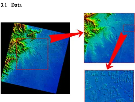
Figure 5. Low resolution DSM of Beijing used in the experiment which contained mountainous terrains with both dramatic and mild topographic relief and flat terrains with large amount of urban buildings.
ZY-3 satellite was launched in 2012. Forward and backward resolution of ZY-3 was 3.5m, and nadir resolution was 2.1m. DSM with GSD of 10-30m generated by dense matching of ZY-3 imagery was used as experiment data in this paper. The experiment area was at Beijing, which contained mountainous ISPRS Annals of the Photogrammetry, Remote Sensing and Spatial Information Sciences, Volume III-3, 2016
terrains with both large and small elevation variation and flat terrains with large amount of urban buildings (Figure 5). 3.2 Experiment Results and Analysis
Progressive morphological filtering (PMF) is a simple yet frequently used method for automatic extraction of DTM from LiDAR datasets, which was used here as a comparison of the proposed method. Visual verification and quantitative comparison between PMF and TSGF are analysed in this section.
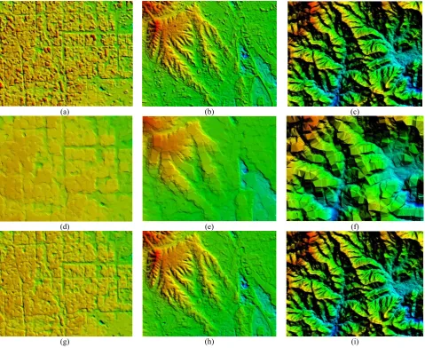
Firstly, results of three typical regions were picked out to visually compare effectiveness of the two methods. The first row in Figure 6 shows DSM of flat terrains (with large amount of non-ground points), mild mountainous terrains (with some non-ground points) and steep mountainous terrains (with no non-ground points), respectively. The second and third row of Figure 6 show results of PMF and TSGF on the above three regions, respectively. From the figure, it is clear that the proposed TSGF is better than PMF especially in mountainous terrains (b and c) since the former filtered the non-ground points as well as kept the terrains while PMF spoiled the terrains.
(a) (b) (c)
(d) (e) (f)
(g) (h) (i)
Figure 6. Visual comparison of DSM and DTM in different terrains. The first row is the DSM in flat terrains with large amount of non-ground points (a), mild mountainous terrains with some non-ground points (b), and steep mountainous terrains (c). The second and the third row are the DTMs processed with PMF and TSGF, respectively.
Secondly, elevation profiles of the results help to compare these two methods, which show more detailed information than visual examination on the results. Figure 7(a) shows the location of the two profiles. Figure 7(b) is the profile1 in Figure 7(a), which located at mild mountainous terrain areas with some non-ground points. This profile indicates that both PMF and TSGF successfully removed non-ground points in this area (red circle in the figure). However, PMF also damaged terrains of mild mountainous area, while TSGF kept the terrains of this location. Figure 7(c) is the profile2 in Figure 7(a), which shows result of
flat area with more non-ground points. Both methods removed non-ground points at this area, however, PMF smoothed the terrains heavier than that of TSGF, which indicated that TSGF works better on filtering of DSM.
Lastly, quantitative analysis of the result was done with the reference of 30m resolution open dataset SRTM (Smith and Sandwell, 1997; Becker et al., 2009). Three indicators were used to analyse the influence on accuracy of DSM by different filtering methods: MAE (Mean Absolute Error), SDE (Standard Deviation of Error) and LP90 (Line Deviations at the 90th ISPRS Annals of the Photogrammetry, Remote Sensing and Spatial Information Sciences, Volume III-3, 2016
percentage). It is noticed that SRTM might has a systematic offset with the ground truth. Therefore, MAE and LDP90 cannot reflect the accuracy of DSM exactly. In comparison, SDE will be more objective for ground filtering. Table 1 shows the results of the three indicators, in which we can find that the accuracy of DTM after processed by PMF was much lower than the original DSM in all three indicators. Meanwhile, the accuracy of DTM processed by TSGF was better than the original DSM. The MAE indicator was slightly lower than the original DSM, however, SDE and LDP90 decreased evidently, which demonstrated the effectiveness of the proposed method.
(a)
(b)
(c)
Figure 7. Visual comparison of DSM and DTM in mountainous terrains (b), and flat terrains(c), by elevation profiles in (a).
MAE/m SDE/m LDP90/m
DSM 10.53 7.55 11.48
DTM(PMF) 12.97 10.79 13.21
DTM(TSGF) 10.44 6.91 10.38
Table 1. Accuracy of DSM and DTM extracted by PMF and TSGF.
Another experiment on the effect of filtering method was done by filtering sampled DSM of the original data into 4 different resolutions: 10m, 15m, 20m and 30m. Accuracy of filtering results showed that the proposed method was effective for the 4
resolutions. However, with more decrease of the resolution, the proposed method would be less useful (Figure 8). It was possibly caused by the lost of land surface objects, which would lead to the effect that the elevation variation of non-ground points on DTM was very small thus not able to be detected.
Figure 8. RMSE of TSGF results with different resolutions. 4. CONCLUSION
Because of small differences between steep terrains and elevation of non-ground points, local filtering methods used for dense LiDAR data are not suitable for low resolution DSM. However, difference in overall characteristic of steep terrains and flat terrains (with non-ground points) makes it possible to remove the non-ground points with non-local filtering method. A two-steps semi-global filtering method was proposed to automatically extracting DTM from DSM. Experiments on DSM produced by dense matching using ZY-3 satellite imagery demonstrated the effectiveness of the proposed method. The proposed method might be used to replace manual editing in DTM production from low resolution DSM.
However, the slope threshold in the proposed method used to detect flat terrains still has some shortcomings. If the threshold is too large, some steep terrains will be detected as flat terrains which might damage the steep terrains, while if it is too small, some non-ground points would not be removed in the processing. Therefore, how to make this threshold adaptive and robust is our future work.
ACKNOWLEDGEMENTS
This work was supported by National Natural Science Foundation of China (Grant No. 41571434, Grant No. 41322010) and National Key Basic Research and Development Program of China (Grant No. 2012CB719904).
REFERENCES
Achanta, R., Shaji, A., Smith, K., Lucchi, A., Fua, P. and Susstrunk, S., 2012, SLIC Superpixels Compared to State-of-the-art Superpixel Methods, IEEE Transaction on Pattern Analysis and Machine Intelligence, 34(11), pp. 2274-2282. Axelsson, P., 2000, DEM generation from laser scanner data using adaptive TIN models. In IAPRS. Vol. 33. Part B4/1, pp. 110-117.
Becker, J. J., D. T. Sandwell, W. H. F. Smith, J. Braud, B. Binder, J. Depner, D. Fabre, J. Factor, S. Ingalls, S-H. Kim, R. Ladner, K. Marks, S. Nelson, A. Pharaoh, G. Sharman, R. Trimmer, J. vonRosenburg, G. Wallace and P. Weatherall., 2009, Global Bathymetry and Elevation Data at 30 Arc Seconds ISPRS Annals of the Photogrammetry, Remote Sensing and Spatial Information Sciences, Volume III-3, 2016
Resolution: SRTM30_PLUS, Marine Geodesy, 32(4), pp.355-371.
Besag, J., 1986, On the Statistical Analysis of Dirty Pictures, Journal of Royal Statistical Society, 48(3), pp. 259-302. Boykov, Y., Kolmogorov, V., 2004, An Experimental Comparison of Min-Cut/Max-Flow Alogorithms for Energy Minimization in Vision. IEEE Transaction on Pattern Analysis and Machine Intelligence, 26(9), pp. 1124-1137.
Chen, Q., Gong, P., Baldocchi, D. and Xie, G., 2007, Filtering airborne laser scanning data with morphological methods, Photogrammetric Engineering and Remote Sensing, 73(2), pp.175–185.
Geiß, C., Wurm M., Breunig, M., Felbier, A, and Taubenböck, H., 2015, Normalization of TanDEM-X DSM Data in Urban Environments With Morphological Filters, IEEE Transaction on Geoscience and Remote Sensing, 53(8), pp. 4348–4361. Gruen, A., 2012, Development and Status of Image Matching in Photogrammetry. Photogrammetric Record, 26(137), pp.36-57. Habib, A. F., Eui-Myoung, K. and Chang-Jae, K., 2007, New methodologies for true orthophoto generation. Photogrammetric Engineering and Remote Sensing, 73(1):25-36.
Hirschmüller, H., 2008, Stereo Processing by Semiglobal Matching and Mutual Information. IEEE Transaction on Pattern Analysis and Machine Intelligence, 30(2), pp. 328-341. Hu, X., Ye L., Pang S. and Shan J., 2015, Semi-Global Filtering of Airborne LiDAR Data for Fast Extraction of Digital Terrain Models, Remote Sensing, 7(8), pp.11996–11015.
Kirkpatrick, S., Gelatt, C., Vecchi, M., 1983, Optimization by simulated annealing, Science, vol. 220, pp. 671–680.
Kraus K. and Pfeifer, N., 1998, Determination of terrain models in wood areas with airborne laser scanner data, ISPRS Journal of Photogrammetry and Remote Sensing, 53(4), pp.193–203. Martha, T. R., Kerle, N., Jetten, V., van Westen, C. J., Vinod Kumar, K. V., 2010. Landslide volumetric analysis using Cartosat-1-Derived DEMs. IEEE Geoscience and Remote Sensing Letters, 7(3), pp.582–586.
Meng, X., Wang, Le, José Luis Silván-Cárdenas, Nate Currit, 2009, A multi-directional ground filtering algorithm for airborne LiDAR, ISPRS Journal of Photogrammetry and Remote Sensing, 64(1), pp.117-124.
Pingel, T. J., Clarke, K. C., and McBride, W. A., 2013, An improved simple morphological filter for the terrain classification of airborne LiDAR data, ISPRS Journal of Photogrammetry and Remote Sensing, 77(3), pp. 21–30. Sithole, G., 2001, Filtering of laser altimetry data using a slope adaptive filter, In IAPRS, vol. 34, pp. 203–210.
Smith, W. H. F., and Sandwell, D. T., 1997, Global seafloor topography from satellite altimetry and ship depth soundings, Science, vol. 277, pp. 1957-1962.
Sreedhar, M., Muralikrishnan, S. and Dadhwal, V.K., 2015, Automatic Conversion of DSM to DTM by Classification Techniques Using Multi-date Stereo Data from Cartosat-1. Journal of Indian Society of Remote Sensing, 43(3), pp. 513-520.
Sun, J., Zheng, N., Shum, H., 2003, Stereo Matching Using Belief Propagation. IEEE Transaction on Pattern Analysis and Machine Intelligence, 25(7), pp.787-800.
Szeliski, R., Zabih, R., Scharstein, D., Veksler O., Kolmogorov, V., Agarwala A., Tappen M. and Rother C., 2006, A comparative study of energy minimization methods for markov random fields. In ECCV, part II, pp.16-29.
Veksler, O., 1999, Efficient graph-based energy minimization methods in computer vision. P.H.D. Thesis, Cornell University, U.S.
Vosselman, G., 2000, Slope based filtering of laser altimetry data, In IAPRS, vol. 33, pp. 935–942.
Vosselman, G., Sithole, G., 2004, Experimental comparison of filtering algorithms for bare-earth extraction from airborne laser scanning point clouds. ISPRS Journal of Photogrammetry and Remote Sensing, 59(1-2), pp. 85-101.
White, S.A., Wang, Y., 2003. Utilizing dems derived from LiDAR data to analyze morphologic change in the North Carolina coastline. Remote Sensing of Environment, 85 (1), pp. 39–47.
Zhan, Z. and Lai, B.,2015, A Novel DSM Filtering Algorithm for Landslide Monitoring Based on Multiconstraints, IEEE Journal of Selected Topics in Applied Earth Observations, 8(1), pp. 324-331.
Zhang, K., Chen, S., Whitman, D., Shyu, M., Yan J., and Zhang C., 2003, A progressive morphological filter for removing nonground measurements from airborne LiDAR data, IEEE Transaction on Geoscience and Remote Sensing, 41(4), pp. 872–882.