BENCHMARKING DEEP LEARNING FRAMEWORKS FOR THE CLASSIFICATION OF
VERY HIGH RESOLUTION SATELLITE MULTISPECTRAL DATA
M. Papadomanolakia∗, M. Vakalopouloua∗, S. Zagoruykob, K. Karantzalosa
a
Remote Sensing Laboratory, National Technical University, Zographou campus, 15780, Athens, Greece
[email protected]; [email protected]; [email protected]
bImagine/Ligm, Ecole des Ponts ParisTech,
Cite Descartes, 77455 Champs-sur-Marne, France [email protected]
Commission VII, WG IV
KEY WORDS:Machine Learning, Classification, Land Cover, Land Use, Convolutional, Neural Networks, Data Mining
ABSTRACT:
In this paper we evaluated deep-learning frameworks based on Convolutional Neural Networks for the accurate classification of multi-spectral remote sensing data. Certain state-of-the-art models have been tested on the publicly availableSAT-4andSAT-6high resolution satellite multispectral datasets. In particular, the performed benchmark included theAlexNet,AlexNet-smallandVGGmodels which had been trained and applied to both datasets exploiting all the available spectral information. Deep Belief Networks, Autoencoders and other semi-supervised frameworks have been, also, compared. The high level features that were calculated from the tested models managed to classify the different land cover classes with significantly high accuracy ratesi.e.,above 99.9%. The experimental results demonstrate the great potentials of advanced deep-learning frameworks for the supervised classification of high resolution multispectral remote sensing data.
1. INTRODUCTION
The detection and recognition of different objects and land cover classes from satellite imagery is a well studied problem in the remote sensing community. The numerous national and commer-cial earth observation programs continuously provide data with different spatial, spectral and temporal characteristics. In order to operationally exploit these massive streams of imagery, ad-vanced processing, mining and recognition tools are required. These tools should be able to timely extract valuable informa-tion regarding the various terrain objects and land cover, land use status.
How automated and how accurate these recognition tools are, is the critical aspect for their applicability and operational use. Re-garding automation, although unsupervised and semi-supervised approaches possess a native advantage, when comes to big data from space with important spatial, spectral and temporal vari-ability, efficient generic tools may be based on supervised ap-proaches which have been trained to handle and classify such datasets [Karantzalos et al., 2015, Cavallaro et al., 2015].
Among supervised classification approaches, Support Vector Ma-chines (SVM) [Vapnik, 1998] and Random Forests [Breiman, 2001] have been broadly used for remote sensing applications [Camps-Valls and Bruzzone, 2009, Tokarczyk et al., 2015]. Un-der supervised frameworks every training dataset must be ade-quately exploited in order to describe compactly and adeade-quately each class. To this end, training datasets may consist of a com-bination of spectral bands, morphological filters [Lefevre et al., 2007], texture [Volpi et al., 2013], point descriptors [Wang et al., 2013], gradient orientation [Benedek et al., 2012],etc.
∗These authors contributed equally to this work.
Patches Deep Models
AlexNet,
VGG,
etc.
Class 1
Class 2
Class 3
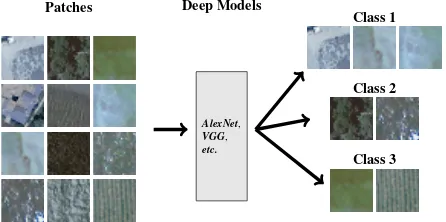
Figure 1: Certain state-of-the-art models have been tested on the publicly availableSAT-4andSAT-6high resolution satellite mul-tispectral datasets. All the models have been designed and trained based on theDeepSatdataset.
Recently, deep learning architectures have gained attention in computer vision and remote sensing by delivering state-of-the-art results on image classification [Sermanet et al., 2013], [Krizhev-sky et al., 2012], object detection [LeCun et al., 2004] and speech recognition [Xue et al., 2014]. Several deep architectures [Deng, 2014, Schmidhuber, 2015] have been employed, with the Deep Belief Networks, Autoencoders, Convolutional Neural Networks and Deep Boltzmann Machines being some of the most com-monly used in the literature for a variety of problems. In partic-ular, for the classification of remote sensing data certain deep ar-chitectures have provided highly accurate results [Mnih and Hin-ton, 2010, Chen et al., 2014, Vakalopoulou et al., 2015, Basu et al., 2015, Makantasis et al., 2015, Marmanis et al., 2016].
training data was released [Basu et al., 2015]. DeepSat con-tains patches extracted from the National Agriculture Imagery Program (NAIP) dataset with about 330,000 scenes spanning the entire Continental United States and approximately 65 terabytes of size. The images consist of 4 bands: red, green, blue and Near Infrared (NIR) and were acquired at a ground sample distance (GSD) of 1 meter, having horizontal accuracy up to 6 meters. The dataset is composed of two discrete units, each of them hav-ing two different group of patches: one for trainhav-ing and one for testing. SAT-4 is the first unit and it has four different classes which are: barren land, trees, grassland and a class that consists of all land cover classes other than the above three. It contains 400.000 training and 100.000 testing patches. The second unit, SAT-6, contains six different classes: barren land, trees, grass-land, roads, buildings and water bodies. It contains 324.000 train-ing and 81.000 testtrain-ing patches. The large number of labelled data thatDeepSatprovides, makes it ideal for benchmarking different deep architectures.
In this paper, motivated by the recent advances on deep convolu-tional neural networks, we benchmark the performance of certain models for classifying multispectral remote sensing data (Fig-ure 1). Based on theDeepSatdataset, we have trained different models and reported on their performances. In particular, Alex-Net,AlexNet-smallandVGGmodels have been implemented and trained on theDeepSatdataset [Krizhevsky et al., 2012, Jader-berg et al., 2015, Ioffe and Szegedy, 2015, Vakalopoulou et al., 2015]. The high accuracy rates demonstrate the potentials of advanced deep-learning frameworks for the supervised classifi-cation of high resolution multispectral remote sensing imagery. Comparing with Deep Belief Networks, Autoencoders and Semi-supervised frameworks [Basu et al., 2015] the proposed here Alex-NetandVGGdeep architectures outperform the state-of-the-art delivering classification accuracy rates above 99.9%.
The remainder of the paper is organized as follows. In Section 2., we briefly describe different deep learning models while in Sec-tion 3. we present and discuss their results. The last secSec-tion pro-vides a short summary of the contributions and examines poten-tial future directions.
2. DEEP-LEARNING FRAMEWORKS
In this section all the tested models and their parameters are pre-sented. Both training and testing datasets had been normalised before inserted into the networks. The implementation of all compared deep learning frameworks was performed in the open source Torch deep learning library [Collobert et al., 2011], while the specific implementation is available in authors’GitHub ac-counts.
2.1 AlexNet-PretrainedNetwork
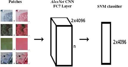
Similar to [Vakalopoulou et al., 2015, Marmanis et al., 2016] the already pretrainedAlexNetnetwork [Krizhevsky et al., 2012] has been employed, here, for feature extraction. In particular, features from the last layer (FC7) were extracted using two spectral band combinations (red-green-blue and NIR-red-green). In this way, a vector with high level features of size2x4096has been created for each patch. Using the training dataset an SVM classifier has been trained (Figure 2) and then the produced model was used for the classification of the testing patches.
The main drawback of this specific setup is the high dimensional-ity of the employed feature vector (i.e.,2x4096) as the pretrained model can not handle more than three spectral bands per patch.
Patches
Figure 2: The FC7 layer of the PretrainedAlexNetnetwork has been employed for extracting features and train a SVM classifier. Two different band combinations (red-green-bue and NIR-red-green) have been formulated in order to exploit all the available spectral information.
2.2 AlexNetNetwork
In order to overcome the previous problem we trained an Alex-NetNetwork using theDeepSatdataset. The model consists of 22 layers: 5 convolutional, 3 pooling, 6 transfer functions, 3 fully connected and 5 dropout and threshold. The model follows the patterns as depicted in Figure 3. More specifically, the first con-volutional layer receives the raw input patch which consists of 4 channels (or input planes) and is of size 28x28. The image is fil-tered with kernels of size 4x3x3 and a stride of 1 pixel, producing an output volume of size 16x26x26. The second layer is a transfer function one which applies the rectified linear unit (ReLU) func-tion element-wise to the input tensor. Thus, the dimensions of the image remain unchanged. Next comes a max pooling layer, which is used to progressively reduce the spatial size of the im-age in order to restrict the amount of network computation and parameters and protect from overfitting. This pooling layer uses kernels of size 2 and a stride of 2, producing an output volume of size 16x13x13.
The next 3 layers follow the same pattern (Convolutional-ReLU-MaxPooling). The Convolutional layer accepts the 16x13x13 volume and produces an output of size 48x13x13 by using 3x3 kernels, with a stride of 1 and a zero padding of 1 pixel. The Convolutional layer is followed by a ReLU and a MaxPooling layer. The latter having kernels of size 3 and a stride of 2 is de-livering output volumes of size 48x6x6. The seventh layer is also a Convolutional layer which delivers an output of size 96x6x6 by applying 3x3 kernels and stride and zero padding of 1. The eighth layer is a ReLU one. Layers 9,10 and 11,12 follow the same pattern (Convolutional-ReLU). The ninth layer is filtering the in-put volume with kernels of size 3x3, with a stride of 1 and zero padding of 1, delivering an output of size 64x6x6. The eleventh convolutional layer uses the same hyperparameters. The twelfth convolutional layer is a maxpooling one, which uses kernels of size 2 and a stride of 2 to produce an output of size 64x3x3.
Input patch
Figure 3: A brief illustration of theAlexNetmodel which was employed here. The network takes as input patches of 4x28x28 (dimen-sions). The network consists of 5 convolutional, 3 fully connected layers and 6 transfer function. A 4 or 6 way soft-max layer is applied depending on the dataset.
of size 4x1, where 4 is the number of class scores. Lastly, we use a soft-max layer with 4 or 6 ways depending on the tested dataset.
Regarding the implementation, we trained the model with a learn-ing rate of 1 for 36 epochs, while every 3 epochs the learnlearn-ing rate was reduced at half. We set the momentum to 0.9, the weight decay parameters to 0.0005 and the limit for the Threshold layer to 0.000001.
2.3 AlexNet-smallNetwork
Another model that we tested was a simpler smallAlexNet Net-work. The model consists of 10 layers. The first layer is a convo-lutional layer and is feeded with the original input image of size 4x28x28, producing a volume of size 32x24x24. In this setup, we did not use the ReLU function but the Tangent one. Con-sequently the Tangent layer comes after the first convolutional one, applying the tangent function element-wise to the input ten-sor. After that, follows a third max pooling layer which narrows down the size of the image from 32x24x24 to 32x8x8. The next 3 layers follow the same pattern and result to an output volume of size 64x2x2. Finally, 4 fully-connected layers follow. At this point we should mention that the model does not contain Dropout layers contrary to the previous fullAlexNetmodel. Nonetheless, results were satisfactory, mostly because of the 2 max pooling layers which made the spatial size of the images smaller and con-troled overfitting.
Finally, the parametrization for theAlexNet-smallwas chosen to be similar with the previous fullAlexNetone. Again we trained the model with a learning rate of 1 for 36 epochs. The learning rate was reduced in half at every 3 epochs. We set the momentum to 0.9 and the weight decay parameters to 0.0005.
2.4 VGGNetwork
Moreover, we experimented with the recentVGGmodel [Jader-berg et al., 2015] which was initially proposed for text recogni-tion. The model consists of 59 levels and it repeatedly makes use of specific layers that include dropout and batch normaliza-tion [Ioffe and Szegedy, 2015]. It should be noted that these two kinds of layers are very important in order to accelerate the entire process and avoid overfitting, as the parameters of each training
layer continuously change. The first group of layers has 4 levels and they have the following pattern: the training model starts with a convolutional layer that takes the input image of size 4x28x28 and it produces an output of size 64x28x28. Then, a batch nor-malization layer is applied with a value of 0.001 added to the standard deviation of the input maps. After that, a ReLU layer is implemented and lastly, a dropout layer with a probability of 0.3. The next group of layers has also 4 levels and it follows the same logic, except the last layer, which is a max pooling one of kernel size 2 and a stride of 2 that converts the input from 62x28x28 to 64x14x14. These two groups of layers are repeatedly used with the same hyperparameters, except dropout which sometimes has a probability of 0.4. The last 7 layers of the entire training model include some fully connected layers.
The deeper architecture of theVGGmodel requires bigger amount of data as well as more training time. For that reason data aug-mentation with horizontal and vertical flips was performed. Fi-nally, the network was trained for 100 epochs, reducing the learn-ing rate in half every 10 epochs.
2.5 Deep Belief Networks, Autoencoders, Semi-supervised frameworks
Last but not least, the aforementioned CNN-based networks were compared with classification frameworks which have been re-cently evaluated in [Basu et al., 2015] for theDeepSatdataset. In particular, approaches based on Deep Belief Networks, Stacked Denoising Autoencoder and a semi-supervised one were employed. The training and testing included both datasets using different pa-rameters, features maps and configurations for each technique. [Basu et al., 2015] concluded that the semi-supervised approach was more suitable for theDeepSatdataset performing 97.95% and 93.92% accuracies for theSAT-4andSAT-6datasets respec-tively.
3. EXPERIMENTAL RESULTS AND EVALUATION
In this section the performed experimental results are presented along with the comparative study. Both training and testing have been performed separately for the two datasets ofSAT-4and SAT-6. For the quantitative evaluation, the accuracy and precision
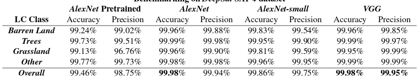
Benchmarking onDeepSat SAT-4dataset
AlexNetPretrained AlexNet AlexNet-small VGG
LC Class Accuracy Precision Accuracy Precision Accuracy Precision Accuracy Precision
Barren Land 99.24% 99.02% 99.96% 99.88% 99.83% 99.54% 99.96% 99.85%
Trees 99.73% 99.51% 99.99% 99.98% 99.95% 99.90% 99.99% 99.97%
Grassland 99.13% 96.76% 99.96% 99.90% 99.81% 99.59% 99.95% 99.99%
Other 99.77% 99.73% 99.98% 99.98% 99.96% 99.95% 99.99% 99.99%
Overall 99.46% 98.75% 99.98% 99.94% 99.86% 99.75% 99.98% 99.95%
Benchmarking onDeepSat SAT-6dataset
AlexNetPretrained AlexNet AlexNet-small VGG
LC Class Accuracy Precision Accuracy Precision Accuracy Precision Accuracy Precision
Barren Land 99.91% 98.72% 99.95% 99.41% 99.96% 99.70% 99.99% 100%
Trees 99.14% 98.78% 99.86% 99.58% 99.77% 99.33% 99.96% 99.87%
Grassland 99.04% 99.72% 99.97% 99.92% 99.95% 99.84% 99.99% 99.96%
Roads 99.16% 96.62% 99.84% 99.61% 99.74% 99.43% 99.89% 99.95%
Buildings 99.92% 98.93% 99.95% 99.08% 99.96% 99.08% 99.99% 99.61%
Water Bodies 100% 100% 100% 100% 99.99% 100% 100% 100%
Overall 99.57% 98.80% 99.93% 99.60% 99.90% 99.56% 99.98% 99.91%
Table 2: Resulting classification accuracy and precision rates after the application of different deep architectures in theSAT-6dataset.
measures have been calculated.
Accuracy= T P+T N
T P+F N+F P+T N (1)
P recision= T P
T P+F P (2)
whereT P is the number of correctly classified patches,T N is the number of the patches that do not belong to the specific class and they were not classified correctly. F N is the number of patches that belong to the specific class but weren’t correctly clas-sified andF Pis the number of patches that do not belong to the specific class but have been wrongly classified.
Regarding the experiments performed on theSAT-4dataset, the calculated precision and accuracy after the application of the dif-ferent deep learning frameworks are presented in Table 1. One can observe that all employed models have obtained quite highly accurate results. More specifically, the overall accuracy rates were in all cases more than 99.4%, while the estimated precision was more than 98.7%. Therefore, the employed deep architec-tures can address the classification task in this particular dataset quite successfully. As expected, the estimated accuracy and pre-cision rates for the PretrainedAlexNetwere lower than the other models, since it was trained on the ImageNet dataset. Moreover, the use of the AlexNet pretrained network makes the computa-tional complexity much higher than in the other models.
The other three models successfully classified all the correspond-ing classes, achievcorrespond-ing accuracy rates more than 99.90%. Addi-tionally, as expected theAlexNetnetwork performs slightly better than theAlexNet-small, which means that the ReLU layer and deeper architectures are more suitable for this specific dataset. In particular, the class that scored lower regarding the accuracy and precision was the grassland, as some patches were misclassified as barren land or trees. TheVGGand theAlexNetmodels resulted into the higher accuracy/precision rates (i.e.,above 99.94%).
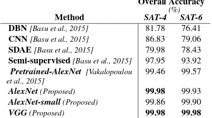
Overall Accuracy
(%)
Method SAT-4 SAT-6
DBN[Basu et al., 2015] 81.78 76.41
CNN[Basu et al., 2015] 86.83 79.06
SDAE[Basu et al., 2015] 79.98 78.43
Semi-supervised[Basu et al., 2015] 97.95 93.92 Pretrained-AlexNet [Vakalopoulou
Table 3: The resulting overall accuracy rates after the application of different learning frameworks for both datasets.
Regarding the experiments performed with theSAT-6dataset, re-sults from the quantitative evaluation are presented in Table 2. As inSAT-4, the pretrainedAlexNet model resulted into the lowest accuracy and precision rates comparing to the other ones. The VGGmodel was the one that resulted into slightly higher ac-curacy rates than theAlexNetandAlexNet-smallmodels. In all cases the overall accuracy rates were higher than 99.6%. More-over, one can observe that thewater bodiesclass was easy to be discriminated from the other ones, as in all cases the calculated accuracy was more than 99.99%. On the other hand, theRoads class was the one that resulted in the lowest accuracy rates as cer-tain misclassification cases occurred with theTreesand Grass-landclasses.
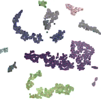
In addition, for the qualitative evaluation of the performed ex-periments thet-SNEtechnique [Van Der Maaten, 2014] was em-ployed.t-SNEhas been tested in different computer vision datasets e.g.,MNIST, NIPS dataset,etc. and it is suitable for the visual-ization of high-dimensional large-real world datasets. In Figure 4 the visualization of the last layer features of theAlexNet-small model for bothSAT-4andSAT-6is shown. In particular, different classes are represented with different colours in the borders of the patches. One can observe that the different classes are well sepa-rated in space, which can justify the high accuracy rates that have been delivered and reported quantitatively in Table 1 and Table 2.
Last but not least, the deep architectures ofAlexNet & VGGwere compared with the recently proposed and evaluated ones from [Basu et al., 2015]. In Table 3, the overall accuracy rates for bothSAT-4andSAT-6 datasets are presented. This benchmark included results after the application of Deep Belief Network (DBN), Convolutional Neural Network (CNN), Stacked Denois-ing Autoencoder (SDAE), a semi-supervised learnDenois-ing framework, AlexNet(pre-trained and small) andVGG. In [Basu et al., 2015], the highest accuracy rates were obtained from the semi-supervised classification framework and were 97.95% and 93.9% for the SAT-4andSAT-6, respectively. As one can observe all the
pro-Evaluating results fromVGGwithout the NIR band
SAT-4 SAT-6
LC Class Accuracy Precision Accuracy Precision
Barren Land 99.96% 98.85% 99.99% 99.89%
Trees 99.99% 99.97% 99.90% 99.64%
Grassland 99.95% 99.99% 99.97% 99.85%
Others 99.99% 99.99% -
-Roads - - 99.99% 99.95%
Buildings - - 99.99% 99.95%
Water Bodies - - 100% 100%
Overall 99.98% 99.95% 99.96% 99.88%
(a) Resulting classes from theSAT-4dataset at the last layer of theAlexNet-smallmodel
(b) Resulting classes from theSAT-6dataset at the last layer of theAlexNet-smallmodel
Figure 4: Qualitative evaluation based on thet-SNE technique. Results from theSAT-4(top) and theSAT-6(bottom) datasets are presented. Different classes are defined with different colours in the borders of the patches. This visualisation corresponds to the last layer of theAlexNet-smallmodel.
posed and applied models in this paper (including the pre-trained AlexNetwhich scored lower that the other ones) outperformed the semi-supervised framework of [Basu et al., 2015]. The proposed deep models efficiently exploited the available spectral informa-tion (all available spectral bands) and created deep features that could accurately discriminate the different classes.
the training process. However, the overall accuracy and precision rates were slightly different, especially on theSAT-6dataset.
4. CONCLUSIONS
In this paper, experimental results after benchmarking different deep-learning frameworks for the classification of high resolution multispectral data were presented. Deep Belief Network (DBN), Convolutional Neural Network (CNN), Stacked Denoising Au-toencoder (SDAE), a semi-supervised learning framework, Alex-Net(pre-trained and small) andVGGwere among the frameworks that were evaluated. The evaluation was based on the publicly availableDeepSatdataset including bothSAT-4andSAT-6. Com-paring with Deep Belief Networks, Autoencoders and Semi- su-pervised frameworks [Basu et al., 2015] the proposed here Alex-NetandVGGdeep architectures outperform the state-of-the-art delivering high classification accuracy rates above 99.9%. The quite promising quantitative evaluation indicates the high poten-tials of deep architectures towards the design of operational re-mote sensing classification tools.
REFERENCES
Basu, S., Ganguly, S., Mukhopadhyay, S., DiBiano, R., Karki, M. and Nemani, R., 2015. DeepSat - A Learning framework for Satellite Imagery. In: ACM SIGSPATIAL.
Benedek, C., Descombes, X. and Zerubia, J., 2012. Building development monitoring in multitemporal remotely sensed image pairs with stochastic birth-death dynamics. Pattern Analysis and Machine Intelligence, IEEE Transactions on 34(1), pp. 33–50.
Breiman, L., 2001. Random forests. Machine Learning 45(1), pp. 5–32.
Camps-Valls, G. and Bruzzone, L., 2009. Kernel Methods for Remote Sensing Data Analysis. Wiley.
Cavallaro, G., Riedel, M., Richerzhagen, M., Benediktsson, J. and Plaza, A., 2015. On understanding big data impacts in re-motely sensed image classification using support vector machine methods. Selected Topics in Applied Earth Observations and Re-mote Sensing, IEEE Journal of PP(99), pp. 1–13.
Chen, Y., Lin, Z., Zhao, X., Wang, G. and Gu, Y., 2014. Deep learning-based classification of hyperspectral data. Selected Top-ics in Applied Earth Observations and Remote Sensing, IEEE Journal of 7(6), pp. 2094–2107.
Collobert, R., Kavukcuoglu, K. and Farabet, C., 2011. Torch7: A Matlab-like Environment for Machine Learning. In: BigLearn, NIPS Workshop.
Deng, L., 2014. A tutorial survey of architectures, algorithms, and applications for deep learning. APSIPA Transactions on Sig-nal and Information Processing.
Ioffe, S. and Szegedy, C., 2015. Batch Normalization: Accelerat-ing Deep Network TrainAccelerat-ing by ReducAccelerat-ing Internal Covariate Shift. In: D. Blei and F. Bach (eds), Proceedings of the 32nd Inter-national Conference on Machine Learning (ICML-15), pp. 448– 456.
Jaderberg, M., Simonyan, K., Vedaldi, A. and Zisserman, A., 2015. Deep Structured Output Learning for Unconstrained Text Recognition. In: International Conference on Learning Repre-sentations.
Karantzalos, K., Bliziotis, D. and Karmas, A., 2015. A scalable geospatial web service for near real-time, high-resolution land cover mapping. Selected Topics in Applied Earth Observations and Remote Sensing, IEEE Journal of PP(99), pp. 1–10.
Krizhevsky, A., Sutskever, I. and Hinton, G. E., 2012. Ima-genet classification with deep convolutional neural networks. In: F. Pereira, C. Burges, L. Bottou and K. Weinberger (eds), Ad-vances in Neural Information Processing Systems 25, Curran As-sociates, Inc., pp. 1097–1105.
LeCun, Y., Huang, F. J. and Bottou, L., 2004. Learning methods for generic object recognition with invariance to pose and light-ing. In: Computer Vision and Pattern Recognition, 2004. CVPR 2004. Proceedings of the 2004 IEEE Computer Society Confer-ence on, Vol. 2, pp. II–97–104 Vol.2.
Lefevre, S., Weber, J. and Sheeren, D., 2007. Automatic building extraction in vhr images using advanced morphological opera-tors. In: Urban Remote Sensing Joint Event, 2007, pp. 1–5.
Makantasis, K., Karantzalos, K., Doulamis, A. and Doulamis, N., 2015. Deep supervised learning for hyperspectral data clas-sification through convolutional neural networks. In: Geoscience and Remote Sensing Symposium (IGARSS), 2015 IEEE Interna-tional, pp. 4959–4962.
Marmanis, D., Datcu, M., Esch, T. and Stilla, U., 2016. Deep learning earth observation classification using imagenet pre-trained networks. IEEE Geoscience and Remote Sensing Letters 13(1), pp. 105–109.
Mnih, V. and Hinton, G., 2010. Learning to detect roads in high-resolution aerial images. In: K. Daniilidis, P. Maragos and N. Paragios (eds), Computer Vision ECCV 2010, Lecture Notes in Computer Science, Vol. 6316, Springer Berlin Heidel-berg, pp. 210–223.
Schmidhuber, J., 2015. Deep learning in neural networks: An overview. Neural Networks 61, pp. 85 – 117.
Sermanet, P., Eigen, D., Zhang, X., Mathieu, M., Fergus, R. and LeCun, Y., 2013. Overfeat: Integrated recognition, localization and detection using convolutional networks. CoRR.
Tokarczyk, P., Wegner, J., Walk, S. and Schindler, K., 2015. Fea-tures, color spaces, and boosting: New insights on semantic clas-sification of remote sensing images. Geoscience and Remote Sensing, IEEE Transactions on 53(1), pp. 280–295.
Vakalopoulou, M., Karantzalos, K., Komodakis, N. and Paragios, N., 2015. Building detection in very high resolution multispec-tral data with deep learning features. In: IEEE International Geo-science and Remote Sensing Symposium (IGARSS),, pp. 1873– 1876.
Van Der Maaten, L., 2014. Accelerating t-SNE Using Tree-based Algorithms. Journal of Machine Learning Research 15(1), pp. 3221–3245.
Vapnik, V. N., 1998. Statistical Learning Theory. Wiley-Interscience.
Volpi, M., Tuia, D., Bovolo, F., Kanevski, M. and Bruzzone, L., 2013. Supervised change detection in VHR images using con-textual information and support vector machines. International Journal of Applied Earth Observation and Geoinformation 20(0), pp. 77 – 85.
Wang, M., Yuan, S. and Pan, J., 2013. Building detection in high resolution satellite urban image using segmentation, corner de-tection combined with adaptive windowed hough transform. In: Geoscience and Remote Sensing Symposium (IGARSS), 2013 IEEE International, pp. 508–511.