A DETAILED STUDY ABOUT DIGITAL SURFACE MODEL GENERATION USING
HIGH RESOLUTION SATELLITE STEREO IMAGERY
K. Gong, D. Fritsch
Institute for Photogrammetry, University of Stuttgart, 70174 Stuttgart (Ke.Gong, dieter.fritsch)@ifp.uni-stuttgart.de
Commission I, WG I/4
KEY WORDS: High Resolution Satellite Images, RPCs, PTE, tSGM, DSM generation
ABSTRACT:
Photogrammetry is currently in a process of renaissance, caused by the development of dense stereo matching algorithms to provide very dense Digital Surface Models (DSMs). Moreover, satellite sensors have improved to provide sub-meter or even better Ground Sampling Distances (GSD) in recent years. Therefore, the generation of DSM from spaceborne stereo imagery becomes a vivid research area. This paper presents a comprehensive study about the DSM generation of high resolution satellite data and proposes several methods to implement the approach. The bias-compensated Rational Polynomial Coefficients (RPCs) Bundle Block Adjustment is applied to image orientation and the rectification of stereo scenes is realized based on the Project-Trajectory-Based Epipolarity (PTE) Model. Very dense DSMs are generated from WorldView-2 satellite stereo imagery using the dense image matching module of the C/C++ library LibTsgm. We carry out various tests to evaluate the quality of generated DSMs regarding robustness and precision. The results have verified that the presented pipeline of DSM generation from high resolution satellite imagery is applicable, reliable and very promising.
1. INTRODUCTION
The Digital Surface Model (DSM) is a common photogrammetric product which is widely applied in the surveying and mapping and Geographic Information System (GIS) area. With the invention of the Semi Global Matching (SGM) algorithm, stereo pairs are matched pixelwise leading to the generation of a very dense DSM from stereo pairs. Moreover, the SGM algorithm is fast and robust to the parameterization (Hirschmüller, 2008). The C/C++ library LibTsgm was developed at the Institute for Photogrammetry, University of Stuttgart and outsourced into the nFrames GmbH in 2013. LibTsgm is also the core library of the software SURE. It is successfully used for airborne and close range photogrammetry (Fritsch, 2015). In February 2013, the European Spatial Data Research Organization (EuroSDR) organized a workshop presenting a benchmark for DSM generation from large frame airborne imagery in the Munich testsite, which provided the first comprehensive overview about competing algorithms (Fritsch, et al., 2013; Haala, 2013). SURE matched high overlapping airborne images at Ground Sampling Distances (GSD) of 10cm stereos by LibTsgm and therefore a very dense DSM of the testsite was available (Haala, 2013).
Remote sensing via satellite imagery becomes a fast and efficient method to acquire the surface information. Since the successful launch of the first Very High Resolution (VHR) satellites like IKONOS in September 1999 or Quickbird in October 2001, the GSDs of satellite sensors are improved over time which started a new age of remote sensing (Maglione et al., 2013). Nowadays, many VHR satellite sensors can provide panchromatic imagery with half meter GSD, such as WorldView-1 and WorldView-2, provided by DigitalGlobe. The latest VHR satellite WorldView-3 launched by DigitalGlobe delivers even WorldView-30cm GSD imagery. Many VHR satellites are also able to provide multi-scene satellite images, which boosts the satellite photogrammetry to new dimensions. As we know, most stereo airborne imagery can
provide a very detailed view of the surface with GSD less than 20cm. Satellite stereo images have the advantages that they can provide sub-meter GSD and their coverage is much larger than those of airborne stereo pairs. Thereby, the VHR satellite imagery becomes a new option to generate the 3D point cloud and DSM. The VHR dataset and reference data used in this paper are introduced in section 2.
In order to generate DSM from VHR satellite stereo images, the orientation of the stereo images is the first essential step. The traditional frame images apply the physical sensor model based on the collinearity condition. This model shows the rigorous relation between image points and corresponding ground points and each parameter has a physical meaning (Jacobsen, 1998). But for the satellite’s situation, the physical model is complicated and it will change with different sensors. Moreover, the parameters, for example like interior elements and exterior elements, are kept confidential by many commercial satellite image providers (Tong, et al., 2010). Instead, the satellite imagery vendors provide 80 Rational Polynomial Coefficients (RPCs) along with the images to the users. Then a generalized model can be derived from the RPCs, which can present the pure mathematic relation between the image coordinates and the object coordinates as a ratio of two polynomials. Some researchers have confirmed that the RPC model can replace the physical model and maintain the accuracy (Grodecki and Dial, 2001; Hanley and Fraser, 2001; Fraser, et al., 2002). The RPC model has also been adopted by the OpenGIS Consortium as a part of the standard image transfer format in 1999 (Tong, et al., 2010). Because the original RPCs provided by image vendors are at low accuracy, if they are directly applied to the bundle block adjustment, there will be discrepancies between the calculated coordinates and the true coordinates (Grodecki and Dial, 2003). In order to remove these discrepancies, a bias compensation for the bundle block adjustment is necessary. Studies have shown, that the bias-compensated RPC block adjustment can provide the orientation ISPRS Annals of the Photogrammetry, Remote Sensing and Spatial Information Sciences, Volume III-1, 2016
results as accurate as the physical camera model (Grodecki and Dial, 2003; Fraser and Hanley, 2005). This paper utilizes the bias-compensated RPC bundle block adjustment to implement the orientation. The general theory is introduced in section 3.1.
If the corresponding points on the stereo pair have no vertical parallaxes, the search range of dense stereo matching will be reduced from 2D space to 1D space and then the processing time will be much decreased (Wang, et al., 2010). An important and significant characteristic of epipolar images is that the corresponding points on the epipolar pair are located on the same row (Pan and Zhang, 2011). Therefore, the image rectification will save much calculating time and possessed memory during dense image matching. In order to attain the epipolar stereo images, the epipolar geometry needs to be established first. For traditional frame cameras, the images are perspective images, which means each image has a unique perspective center and the intersection of the epipolar plane and each perspective image plane forms the epipolar lines (Loop and Zhang, 1999). In contrast to perspective stereo images, the VHR satellite pushbroom sensors are difficult to establish the epipolar geometry. Because the perspective center and the attitude of each scanning line of the pushbroom sensor are changing during the scanning. Some approximate models have been developed to solve this problem such as Direct Linear Transformation (DLT) and parallel projection (Wang, 1999; Morgan, et al., 2006). Kim (2000) has investigated the epipolar geometry established by the cameras moving with constant velocity and altitude in a trajectory. And the key procedure of this epipolar geometry is to find a proper model that can establish the geometric relationship between the image and object space. As we know, the relationship between object and image space is built as a simple mathematic projection by the RPC model. Thus, the trajectory epipolar geometry supported by the RPC model is selected to generate the epipolar image pairs for the VHR satellite data, which is also called the projection-trajectory-based epipolarity (PTE) model (Wang, et al., 2010). Among the alternative models, the PTE model is the simplest model to describe the epipolar geometry. More introduction will be presented in section 3.2.
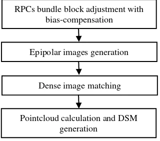
Figure 1. Overview of the workflow
Nowadays, matching algorithms mainly aim on the dense image matching which conducts a very dense and pixel-wise match. Its biggest benefit is that the GSD of generated 3D point cloud is the same as the original stereo images (Haala, 2013). Recently, researchers have investigated and verified the availability and reliability of the dense stereo matching approach with VHR satellite imagery (Reinartz, et al., 2010; d’Angelo and Reinartz, 2011; Wohlfeil, et al., 2012). This paper applies the C/C++ library LibTsgm to implement the dense image matching and deliver the disparity images. The core algorithm of LibTsgm is
the modified Semi-Global Matching approach (tSGM), which reduces the computing time and optimizes the memory efficiency (Fritsch, et al. 2013). The algorithm implements a hierarchical coarse-to-fine method to limit the disparity search ranges. When the higher resolution pyramids start the matching, the results generated from lower resolution pyramids are used as the disparity priors, which can derive search ranges for each pixel. The search ranges’ size will change according to the requirements (Rothermel, et al., 2012). The dense image matching algorithm is described in section 3.3. The epipolar stereo pairs produce the disparity maps by tSGM. These disparity images are eventually fused to generate the 3D point cloud and DSM. An overview of the whole pipeline is given in Fig. 1.
This paper aims at building a pipeline to implement the 3D reconstruction of VHR imagery. The results will be presented in section 4. All the procedures and analysis conducted in this paper are implemented by self-coded programs.
2. DATA DESCRIPTION
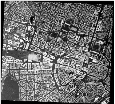
The test VHR satellite stereo imagery is provided by the Deutsches Zentrum für Luft und Raumfahrt (DLR), Oberpfaffenhofen. In all, four WorldView-2 satellite images are made available so that two pairs of stereo images could be processed. The imagery is generated on July 12, 2010, and delivered at Level 1B, which means the images are radiometrically and sensor corrected, but without the map projection. The image pair comprises the main urban area of Munich at 0.5m GSD. In order to compare with the reference data, a subset test area is extracted from the original stereo images. The size of the subset image is 6000*6000 pixels, and the overlapping rate is over 90%. An example of the subset stereo images is shown in Fig. 2.
Figure 2. WorldView-2 stereo image of Munich
Figure 3. Munich aireal photography DSM
The Worldview-2 dataset also provided the RPCs for each image but no Ground Control Points (GCPs). Most GCPs’ coordinates are in the Gauss-Krueger coordinate system based on Bessel ellipsoid. But satellite imagery applies coordinates in the UTM Epipolar images generation
Dense image matching
Pointcloud calculation and DSM generation
RPCs bundle block adjustment with bias-compensation
coordinate system with the WGS84 ellipsoid. Therefore, GCPs are generated manually with the orthophotos at 20cm GSD and using a LiDAR Digital Elevation Model (DEM) at 50cm GSD (see Fig. 3a), provided by the National Mapping Agency of Bavaria (LDBV). The locations of GCPs are selected by using the software ArcMap and interpolated in the DEM by Matlab code. GCPs are selected from the points located on the ground, such as road intersections, tips of zebra lines or corners of playgrounds. The reference data is the aerial photography DSM at 10cm GSD organized by the EuroSDR benchmark “High Density Image Matching for DSM Computation”, which is shown in Fig. 3.
3. PRINCIPLES
3.1 Satellite Image Orientation
The RPC model can build a direct relationship between an image point and the corresponding object point independent to the sensors. It is a pure mathematical model, i.e. it means every coefficient has no physical meaning. Taking the RPCs’ weak accuracy into account, a bias compensation is necessary for the adjustment to reduce the systematic errors. Here we give a cursory introduction about the model, and the functions are following Grodecki and Dial (2003). A comprehensive form of the bias-compensated RPC model is presented in 3.1.
( , , )
where l and s are the line and sample coordinates in the image space, which presents the rows and columns. Functions NumL, DenL, Nums and Dens are the cubic polynomial functions composed by the 80 RPCs, the normalized object coordinates (latitude B, longitude L and elevation H). εL and εS are random errors. Adjustment functions Δp and Δr describe the bias compensation for the image coordinates calculated via the original RPC model. A polynomial function is selected in this paper to implement the bias-compensation, as shown in 3.2.
0 parameters. The parameters a0 and b0 absorb the offsets, and the parameters aL, aS, bL and bS can absorb the drift effects. The high-order elements are used to remove small effects caused by other systematic errors (Grodecki and Dial, 2003; Fraser and Hanley, 2005). When the image coverage is small, the influence of higher order parameters is negligible (Fraser, et al., 2002). Therefore, expansion first. Then its solution can be carried out by applying the least-squares method of parameter estimation.
3.2 Image Rectification
The epipolar geometry of linear pushbroom satellite sensors can be defined as a pure mathematical model which is called the
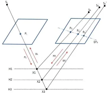
Project-trajectory-based Epipolarity Model or PTE model (Wang, et al., 2010). Fig. 4 is a sketch to show the project trajectory of the PTE model.
Figure 4. Epipolar geometry of satellite stereo images
SL is the perspective center of left image point PL, and PL can be projected to the object space. For example, the image point PL has three corresponding projected points X1, X2 and X3 on three given elevation levels H1, H2 and H3. All of these projected points in the object space can be back-projected to the right image. Then the back-project ray will intersect the right image as a result of three image points PR, PR’ and PR’’, which refer to three perspective centers SR, SR’ and SR’’. The straight line EPR on the right image plane is simulated by the back-projected image points, which is called the quasi-epipolar line. Symmetrically, PR is projected to the elevation levels in the object space and then back-projected to the left image. The corresponding quasi-epipolar line on the left scene is attained. Previous researches have pointed out, that the epipolar line of satellite images is not a straight line but more like a hyperbola. But when the image coverage is small, the influence of the error caused by the simulation is negligible. In this case, the epipolar curve can be simply simulated as a straight line (Kim, 2000; Habib, et al., 2005; Wang, M., et al., 2011). In this paper, each epipolar curve is approximated by an individual straight line in the whole image.
The RPC model is selected to build the projection relations between the object and image coordinates. In Fig. 4, four simplified descriptions FL, BR, FR, and BL are used to implement the image-to-object and the backward projection:
FL: (Line, Sample, Height) --> (Latitude, Longitude)
BR: (Latitude, Longitude, Height) --> (Line, Sample)
FR: (Line, Sample, Height) --> (Latitude, Longitude)
BL: (Latitude, Longitude, Height) --> (Line, Sample)
According to the epipolar geometry defined by the PTE model, the rectified images are resampled via bicubic interpolation. The resampling is undertaken pixel by pixel along every epipolar line on the original stereo images.
3.3 Modified Semi-Global Matching
The Semi-Global Matching method (Hirschmüller, 2008) is a pixelwise image matching method using the Mutual Information (MI) (Viola and Wells, 1997) to calculate the matching costs. A quick review about the SGM algorithm is given first, and the ISPRS Annals of the Photogrammetry, Remote Sensing and Spatial Information Sciences, Volume III-1, 2016
modified Semi-Global Matching is introduced later. All the functions in this chapter follow the work of Rothemel, et al. (2012). The base image is Ib, and the matching image is Im. If the epipolar geometry is known, the potential correspondences will be located in the same row on two images with disparities D. The disparities are estimated such, that the global cost function is minimized. This is just an approximate minimum, and the global cost function is presented in 3.3:
1
Here, the first part of the function is the data term C(p, Dp), which is the sum of all pixel matching costs of the disparities D. The second part represents the constraints for the smoothness composed by two penalizing terms. Parameter n denotes the pixels in the neighborhood of pixel p. T is the operator which equals 1, if the argument is true, otherwise 0. P1 and P2 are the penalty parameters for the small and large disparity changes. The local cost of each pixel C(p,d) is calculated and the aggregated cost S(p,d) is the sum of all costs along the 1D minimum cost paths. The cost paths end at pixel p from all directions and with disparity d. The cost path is presented in 3.4.
1 1
Lri is the cost on image i and along path ri at disparity d. C(p,d) is the matching cost, and the following items are the lowest costs including penalties of the previous pixel along path ri. The last item of the equation is the minimum path cost of the previous pixel of the whole term, which is the subtraction to control the value of Lri in an acceptable size. This subtracted item is constant for all the disparities of pixel p, so the maximum value of Lri is Cmax(p,d) + P2. Then summing up the costs from the paths of all directions, the aggregated cost is presented in 3.5. Finally, the disparity is computed as the minimum aggregated cost.
( , ) ( , ) insensitive to parametrization and provides robust results. It also has a good performance in time and memory consumption. The tSGM applies the disparities to limit the disparity search range for the matching of subsequent pyramid levels (Rothemel, et al.,
2012). Assume Dl is the disparity image generated from the image pyramid l. If pixel p is matched successfully, the maximum and minimum disparities of p are dmax and dminand they are contained in a derived small searching window. If p is not matched successfully, a large search window is used to search dmax and dmin. The search range is stored in two additional images
Rlmax and Rlmin. Images Dl, Rlmax and Rlmin will determine the
disparity search range for the next pyramid level’s dense image matching. As a result, the search range of image pyramid level l-1 is [2*(p+d- dmin), 2*(p+d+ dmax)], which gives a limitation of the search range and saves the computing time and memory. SURE implements an enhanced equation to calculate the path cost, which is presented in 3.6. While the costs of neighboring pixels might be only partly overlapping or even not overlap, here the terms Lr(p-ri, d+k) are ignored. Instead, the bottom or top elements of the neighboring cost Lri(p − ri, dmin (p − ri)) and Lri(p
− ri, dmax (p − ri)) are employed.
In LibTsgm, the penalty parameter P2 adapts smoothing based on a canny edge image. If an edge was detected, low smoothing using P2= P21 is applied. On the contrary, an increased smoothing is forced by setting P2= P21 + P22.
4. EXPERIMENTS
4.1 Bias-compensated RPC Bundle Block Adjustments
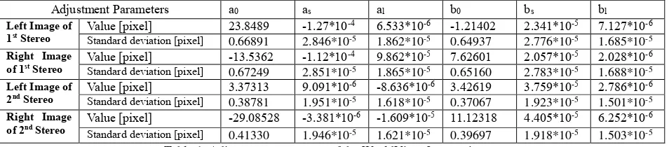
The WorldView-2 imagery has two pairs of stereo images covering the Munich testsite, for which 61 GCPs and 30 check points were employed. Conducting the bias-compensated RPC bundle block adjustment simultaneously for the stereo images, the adjusted parameters are shown in Table 1. Additionally, Table 2 demonstrates the maximum errors and the Root Mean Square (RMS) errors of the back projected image coordinates of the check points. Finally the accuracy of check points’ object coordinates is shown in Table 3.
Table 1 exhibits the adjustment parameters for WorldView-2 stereo imagery and their precisions. As Table 1 displays, the shift parameters a0 and b0 will be the main factors for the orientation when the image size is less than 10,000*10,000pixels. According to the standard deviation, the shift parameters are more precise than the drift parameters al, bl, as,and bs. In table 2, line and sample coordinates represent the coordinates in row and column direction. According to Table 2, all the maximum errors of image coordinates are at sub-pixel level. The RMS error of image coordinates is smaller than 0.3 pixel. In Table 3 it can be seen, that the max error of longitude is over 1m and the maximum height error is 2m. But the RMS error of longitude and latitude are less than 0.4m, the RMS error of elevation is less than 0.7m. The accuracy of the orientation is limited by the accuracy of the GCPs, and it can be improved in the follow-up study. Generally, the bias-compensated RPC bundle block adjustment can provide precise results for subsequent processing.
Table 1. Adjustment parameters of the WorldView-2 stereo image
Adjustment Parameters a0 as al b0 bs bl
Left Image of
1st Stereo Value [pixel] 23.8489 -1.27*10
-4 6.533*10-6 -1.21402 2.341*10-5 7.127*10-6
Standard deviation [pixel] 0.66891 2.846*10-5 1.862*10-5 0.64937 2.776*10-5 1.685*10-5
Right Image
of 1st Stereo Value [pixel] -13.5362 -1.12*10
-4 9.862*10-5 7.62601 2.057*10-5 2.028*10-6
Standard deviation [pixel] 0.67249 2.851*10-5 1.865*10-5 0.65160 2.783*10-5 1.688*10-5
Left Image of
2nd Stereo Value [pixel] 3.37313 9.091*10
-6 -8.636*10-6 3.42619 3.759*10-5 2.786*10-6
Standard deviation [pixel] 0.38781 1.951*10-5 1.618*10-5 0.37067 1.923*10-5 1.501*10-5
Right Image
of 2nd Stereo Value [pixel] -29.08528 -3.381*10
-6 -1.609*10-5 11.12318 4.405*10-5 6.252*10-6
Standard deviation [pixel] 0.41330 1.946*10-5 1.621*10-5 0.39697 1.918*10-5 1.503*10-5 ISPRS Annals of the Photogrammetry, Remote Sensing and Spatial Information Sciences, Volume III-1, 2016
Left image of 1st Stereo Right image of 1st Stereo
line sample line sample
Max Error [pixel] 0.1474 0.6171 0.1451 0.6174
RMS [pixel] 0.0729 0.3077 0.0733 0.3077
Left image of 2nd Stereo Right image of 2nd Stereo
line sample line sample
Max Error [pixel] 0.1296 0.5476 0.1291 0.5472
RMS [pixel] 0.0648 0.2696 0.0648 0.2695
Table 2. Image Reprojection Errors of WorldView-2 Stereo Image
Latitude Longitude Height Max Error [m] 0.5697 1.3524 2.0012 RMS [m] 0.2198 0.3991 0.6988
Table 3. Accuracy of WorldView-2 Stereo Image Covering Munich Test Field
4.2 Epipolar images generation
The following experiment is designed to verify the epipolar geometry accuracy of PTE model. First of all, 25 pairs of corresponding points are selected from the GCPs as check points in the Munich test field. These points are scattered in the images and their image coordinates are considered as the true location in image space. As chapter 3.2 has introduced, the check points’ image coordinates on the left image are projected to the object space and back-projected to the right image. The quasi-epipolar line on the right image is simulated by the back-projected points. The distance between the quasi-epipolar line and the corresponding coordinates of the check points on the right scene are calculated, and the results are demonstrated in Fig. 5 and Fig. 6. The discrete points represent the distribution of the distance between the true conjugate points and the quasi-epipolar line and the bottom of each graph shows the RMS error.
Figure 5. Distance between conjugate points and the quasi-epipolar line of 1st stereo image pair
Figure 6. Distance between conjugate points and the quasi-epipolar line of 2nd stereo image pair
According to Fig. 5 and 6, the distances between the true conjugate points and the quasi-epipolar line for both stereo pairs are below 1 pixel. Moreover, the RMS error of the distances for two image pairs are 0.5 pixel. As the results have shown, we can
consider that the conjugate points are located on the quasi-epipolar line or very near to it.
According to the definition of the PTE model, the epipolar images for the WorldView-2 stereo images are resampled along each epipolar line pixel by pixel. An example epipolar pair is shown in Fig 7.
Figure 7. An example of WorldView-2 epipolar image pair
4.3 Dense Image Matching and DSM Generation
The generated epipolar images are the input for LibTsgm, and the disparity images are delivered as a result. According to the disparity images, the object coordinates for each pixel can be calculated by applying forward intersections. Finally, a DSM of 1m GSD (as Figure 8 shows) is generated by LibTsgm from the WorldView-2 point cloud.
Figure 8: WorldView-2 DSM at 1m GSD
-1 -0,8 -0,6 -0,4 -0,20 0,2 0,4 0,6 0,81
1 3 5 7 9 11 13 15 17 19 21 23 25
Ve
rt
ic
al
P
ar
al
lax
(pi
xe
l)
RMS = 0.501 pixel
-1 -0,8 -0,6 -0,4 -0,20 0,2 0,4 0,6 0,81
1 3 5 7 9 11 13 15 17 19 21 23 25
Ve
rt
ic
al
P
ar
al
lax
(
p
ixe
l)
RMS = 0.499 pixel
Two examples of the reconstructed details are shown in Fig. 9, the left side is the reconstructed point cloud and the right image is the corresponding area on the orthophoto. According to Fig 9. (a) and (b), Munich’s main train station is rebuilt and some textures on the top of the station are reconstructed successfully. In Fig 9. (c) and (d), the trees are reconstructed but the lawn is not. This is a result of the insufficient texture which is challenging for the dense matching process. According to Fig. 9, the generated DSM can describe the terrain with some detail textures and most buildings, streets and vegetation in the city are reconstructed clearly.
(a) (b)
(c) (d)
Figure 9. Detail comparison between DSM and orthophoto
More quantitative analyses are conducted with the reconstructed DSM from the aerial photography and satellite imagery. Here, 20 check points on the ground and 20 check points on the roofs are selected from the aerial photography DSM.
Figure 10. Height difference with the aerial photography DSM (a) ground points (b) roof points
Fig. 10 displays a comparison for the heights of the reconstructed DSM and the aerial photography DSM. As shown, the RMS of the points on the ground is 0.406m (Fig. 10a) and the roof points’ RMS error is 0.972m (Fig. 10b). Moreover, the maximum error of the points on the ground is less than 1m but the maximum error of roof points is larger than 2m. Therefore, the dense image matching algorithm can match the points on the ground better than the points along the roof. The possible reason might be the cast shadow of the buildings. In order to verify this, the following test is conducted.
(a) (b)
(c) (d)
(e) (f)
(g)
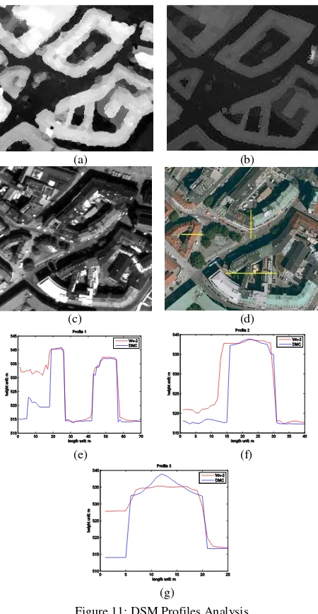
Figure 11: DSM Profiles Analysis
A subsection area of the DSMs generated from satellite imagery and airborne photography are separately shown in Fig. 11 (a) and (b). Comparing the reference airborne photography DSM with the satellite data’s DSM, the boundary of the buildings are sharper. The corresponding area on the original satellite image is depicted in Fig. 11 (c). It is visible, that the side of the building which is covered by a cast shadow performs worse than other sides. The boundary between the buildings and streets have clearer results when there is no shadow at all. Moreover, three height profiles are extracted from the test area. The profiles on the orthophoto is shown in Fig. 11 (d). Comparing the height differences of the profiles on the reconstructed DSM and the aerial photography DSM, the results are shown in Fig 11 (e), (f)
-0,8 -0,6 -0,4 -0,2 0 0,2 0,4 0,6 0,8
1 3 5 7 9 11 13 15 17 19
H
e
ig
ht
D
if
fe
re
nc
e
(
m
)
(a) rms=0.406m
-3 -2 -1 0 1 2 3
1 3 5 7 9 11 13 15 17 19
H
e
ig
ht
D
if
fe
re
nc
e
(
m
)
(b) rms=0.972m
and (g). The red lines in Fig. 11 (e), (f) and (g) present the DSM generated from Worldview-2 stereo images, and the blue lines present the DSM generated by aerial photography with the DMC II 230 camera. As profile 1 and 2 display, the main structure of the buildings is reconstructed clearly. The texture information on the roof is missed in profile 3. According to Fig. 11 (c), and (d), the left part of the buildings in profile 1, 2 and 3 are covered by the cast shadow. It is visible in Fig 11 (e), (f) and (g), that the points on the shadow side of the building have height errors even larger than 15m. In contrast, two different DSM fit well on the side without shadow. Therefore, the shadow has some effect on the reconstruction and will cause some huge errors.
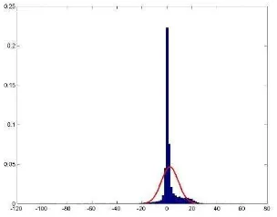
The distribution of the elevation differences is depicted as a histogram presented in Fig 12. The blue bars in Fig 12 are the distribution of the errors and the red line presents the normal distribution with same mean value and standard deviation of the height difference. Here, median, the normalized median deviation (NMAD), 68% and 95% quantiles of absolute error are selected for the results’ robustness estimation. Table 4 displays the statistic evaluation result.
Figure 12: Histogram of the Height differences
Median (m) NMAD (m) Aq68 (m) Aq95 (m)
0.601 1.421 2.241 17.676
Table 4. Robustness Analysis Result
The distribution displayed in Fig 12 shows, that most points are generated with small elevation errors, but still there exist outliers in the DSM. To be more specific, the median of the height difference between DSM generated by satellite imagery and the reference DSM is 0.6m according to Table 4. The NMAD is 1.421m and 68% points of the whole DSM have the evaluated errors less than 2.25m. The 95% quantiles is 17.676m, which is mainly caused by the cast shadow of the buildings. The estimated results indicate, that the 3D Reconstruction pipeline for high resolution satellite data can generate the DSM with acceptable accuracy and robustness.
5. CONCLUSIONS
The RPC Bundle Block Adjustment with additional parameters is applied to process VHR satellite stereo images. This method is proved as a convenient, direct and accurate way to handle VHR satellite data. Generally, the discrepancies of the bias-compensated RPC bundle block adjustment can reach sub-pixel level in image space and sub-meter level in object space. Therefore, the RPC Bundle Block Adjustment provide accurate orientation for post procedures.
The PTE model replaces the traditional physical model perfectly for the linear push broom sensors. In order to define the epipolar
geometry, the RPC model is also utilized to build the relation between object and image space. Although the epipolar curves are not straight lines exactly but hyperbola curves, in our case, they are just approximated by straight lines. This means, we generate every epipolar line with individual parameters and resample the rectified images. The corresponding points of the epipolar pair have sub-pixel vertical parallaxes.
It has been verified in this paper, that the C/C++ library LibTsgm’s base dense matching algorithms are capable to process VHR satellite data. The 3D reconstruction from VHR satellite imagery has been proved as a reliable and robust method. The generated 3D point cloud and DSM are very dense, and the main texture information of the test sites are reconstructed. The DSM has some outliers and some buildings’ boundaries are not sharp because of the shadow’s influence. There is still room to improve the accuracy in some follow-up studies. If there are more stereo pairs, the effect of shadow will be reduced. All in all, the VHR satellite imagery’s DSM generation is quite promising and further research will be done working with WorldView-2 and even the latest WorldView-3 satellite imagery.
ACKNOWLEDGEMENTS
The authors are grateful to DLR Oberpfaffenhofen providing the WorldView-2 stereo imagery and to the LDBV Munich for offering the Munich orthophoto. For the support of using LibTsgm, the advice of nFrames GmbH, Stuttgart is acknowledged.
REFERENCES
d’Angelo, P., Reinartz, P., 2011. Semiglobal matching results on the ISPRS stereo matching benchmark. Report on ISPRS Workshop “High-Resolution Earth Imaging for Geospatial Information”, Hannover, Stuttgart.
Fraser, C., Hanley, H., Yamakawa, T., 2002. Three‐dimensional geopositioning accuracy of Ikonos imagery. The Photogrammetric Record, 17(99), pp. 465-479.
Fraser, C., Hanley, H., 2005. Bias-compensated RPCs for sensor orientation of high-resolution satellite imagery. Photogrammetric Engineering & Remote Sensing, 71(8), pp. 909-915.
Fritsch, D., Becker, S., Rothermel, M., 2013. Modeling Facade Structures Using Point Clouds from Dense Image Matching. Proceedings Intl. Conf. Advances in Civil, Structural and Mechanical Engineering, Inst. Reserach Eng. and Doctors, pp. 57-64.
Fritsch, D., 2015. Some Stuttgart Highlights of Photogrammetry and Remote Sensing. In: Photogrammetric Week ’15, Ed. D.Fritsch, Wichmann/VDE, Berlin and Offenbach, pp. 3-20.
Förstner, W., 1986. A feature based correspondence algorithm for image matching. International Archives of Photogrammetry and Remote Sensing, 26(3), pp. 150-166.
Grodecki, J., Dial, G., 2001. IKONOS geometric accuracy, Proceedings of Joint International Workshop on High Resolution Mapping from Space, Hannover, Germany, pp. 77-86 (CD-ROM).
Grodecki, J., Dial, G., 2003. Block Adjustment of High-Resolution Satellite Images Described by Rational Polynomials. Photogrammetric Engineering & Remote Sensing, 69(1), pp. 59-58.
Haala, N., 2013. The Landscape of Dense Image Matching Algorithms. IN: Photogrammetric Week’13, Ed. D. Fritsch, Wichmann/VDE Verlag, Berlin/Offenbach, pp. 271-284.
Habib, A., Morgan, M., Jeong, S., Kim, K., 2005. Epipolar geometry of line cameras moving with constant velocity and attitude. Electronics and Telecommunications Research Institute Journal 27 (2), pp. 172–180.
Hanley, H., Fraser, C., 2001. Geopositioning Accuracy of IKONOS Imagery: Indication from Two Dimensional Transformations. Photogrammetric Record, 17(98), pp. 317-329.
Hirschmuller, H., 2008. Stereo processing by semiglobal matching and mutual information. Pattern Analysis and Machine Intelligence, IEEE Transactions on, 30(2), pp. 328-341.
Jacobsen K., Block adjustment [J], 1998, Institut for Photogrammetry and Surveying Engineering, University of Hannover.
Kim, T., 2000. A study on the epipolarity of linear pushbroom images. Photogrammetric Engineering and Remote Sensing, 62(8), pp. 961-966.
Loop, C. and Zhang, Z., 1999. Computing rectifying homographies for stereo vision. In: Computer Vision and Pattern Recognition. IEEE Computer Society Conference on, Vol. 1, pp. 2 vol. (xxiii+637+663).
Maglione, P., Parente, C., Vallario, A., 2013. Using Worldview‐ 2 Satellite Imagery to support Geoscience Studies on Phlegraean Area. American Journal of Geosciences, 3 (1), Published Online: http://www.thescipub.com/ajg.toc.
Morgan, M., Kim, K. O., Jeong, S., Habib, A., 2006. Epipolar resampling of space-borne linear array scanner scenes using parallel projection. Photogrammetric Engineering & Remote Sensing, 72(11), pp. 1255-1263.
Pan, H., Zhang, G., 2011. A general method of generating satellite epipolar images based on RPC model. Geoscience and Remote Sensing Symposium (IGARSS), 2011 IEEE International, pp. 3015-3018.
Reinartz, P., d’Angelo, P., Krauss, T., and Chaabouni -Chouayakh, H., 2010. DSM Generation and Filtering from High Resolution Optical Stereo Satellite Data, Proceedings 30th European Association Remote Sensing Laboratories (EARSeL) Symposium, Paris, France, pp. 527-536.
Rothermel, M., Wenzel, K., Fritsch, D., Haala, N., 2012. Sure: Photogrammetric surface reconstruction from imagery. In Proceedings LC3D Workshop, Berlin, pp. 1-9.
Tong, X., Liu, S., Weng, Q., 2010. Bias-corrected rational polynomial coefficients for high accuracy geo-positioning of QuickBird stereo imagery. ISPRS Journal of Photogrammetry and Remote Sensing, 65(2), pp. 218-226.
Viola, P., Wells III, W. M., 1997. Alignment by maximization of mutual information. International journal of computer vision, 24, pp. 137-154.
Wang, M., Hu, F., Li, J., 2010. Epipolar arrangement of satellite imagery by projection trajectory simplification. The Photogrammetric Record, 25(132), pp. 422-436.
Wang, M., Hu, F., Li, J., 2011. Epipolar resampling of linear pushbroom satellite imagery by a new epipolarity model. ISPRS Journal of Photogrammetry and Remote Sensing, 66 (3), pp. 422-436.
Wang, Y., 1999. Automated triangulation of linear scanner imagery. In Joint Workshop of ISPRS WG I/1, I/3 and IV/4 on Sensors and Mapping from Space, pp. 27-30.
Wohlfeil, J., Hirschmüller, H., Piltz, B., Börner, A., Suppa, M., 2012. Fully automated generation of accurate digital surface models with sub-meter resolution from satellite imagery [J]. Int. Arch. Photogramm. Rem. Sens. Spatial Inf. Sci. 34-B3: pp. 75-80.
Zabih, R., Woodfill, J., 1994. Non-parametric local transformsfor computing visual correspondence. In: J.-O. Eklundh (ed.), Computer Vision ECCV ’94, Lecture Notes in Computer Science, Vol. 801, Springer Berlin Heidelberg, pp. 151–158. Zhao, D., Yuan, X., Liu, X., 2008. Epipolar Line Generation from IKONOS Imagery Based on Rational Function Model. The International Archives of the Photogrammetry, Remote Sensing and Spatial Information Sciences. Vol. XXXVII. Part B4: pp. 1293-1297.