GLOBAL AND LOCAL SPARSE SUBSPACE OPTIMIZATION FOR MOTION
SEGMENTATION
Michael Ying Yanga, Sitong Fengb, Hanno Ackermannb, Bodo Rosenhahnb
a
Computer Vision Lab, TU Dresden, Germany
bInstitute for Information Processing (TNT), Leibniz University Hannover, Germany
[email protected], [email protected]
Commission WG III/3
KEY WORDS:Motion segmentation, affine subspace model, sparse PCA, subspace estimation, optimization
ABSTRACT:
In this paper, we propose a new framework for segmenting feature-based moving objects under affine subspace model. Since the feature trajectories in practice are high-dimensional and contain a lot of noise, we firstly apply the sparse PCA to represent the original trajectories with a low-dimensional global subspace, which consists of the orthogonal sparse principal vectors. Subsequently, the local subspace separation will be achieved via automatically searching the sparse representation of the nearest neighbors for each projected data. In order to refine the local subspace estimation result, we propose an error estimation to encourage the projected data that span a same local subspace to be clustered together. In the end, the segmentation of different motions is achieved through the spectral clustering on an affinity matrix, which is constructed with both the error estimation and sparse neighbors optimization. We test our method extensively and compare it with state-of-the-art methods on the Hopkins 155 dataset. The results show that our method is comparable with the other motion segmentation methods, and in many cases exceed them in terms of precision and computation time.
1 INTRODUCTION
In the past years, dynamic scenes understanding has been receiv-ing increasreceiv-ing attention especially on the movreceiv-ing camera or mul-tiple moving objects. Motion segmentation as a part of the video segmentation is an essential part for studying the dynamic scenes and many other computer vision applications (Yang and Rosen-hahn, 2014). Particularly, motion segmentation aims to decom-pose a video into different regions according to different moving objects that tracked throughout the video. In case of feature ex-traction for all the moving objects from the video, segmentation of different motions is equivalent to segment the extracted feature trajectories into different clusters. One example of feature-based motion segmentation is presented in Fig. 1.
Figure 1: Example results of the motion segmentation on the real traffic video from the Hopkins 155 dataset (Tron and Vidal, 2007).
Generally, the algorithms of motion segmentation are classified into 2 categories (Dragon et al., 2012): affinity-based methods and subspace-based methods. The affinity-based methods focus on computing the correspondences of each pair of the trajectories, whereas the subspace-based approaches use multiple subspaces to model the multiple moving objects in the video and the seg-mentation of different motions is accomplished through subspace clustering. Recently, some affinity-based methods (Dragon et al., 2012, Ochs et al., 2014) are proposed to cluster the trajectories with unlimited number of missing data. However, the computa-tion times of them are so high that require an optimizing platform to be reduced. Whereas, the subspace-based methods (Elham-ifar and Vidal, 2009, Ma et al., 2007) have been developed to
reconstruct the missing trajectories with their sparse representa-tion. The drawback is that they are sensitive to the real video which contains a large number of missing trajectories. Most of the existing subspace-based methods still fall their robustness for handling missing features. Thus, there is an intense demand to explore a new subspace-base algorithm that can not only segment multiple kinds of motions but also handle the missing and cor-rupted trajectories from the real video.
ContributionsWe propose a new framework with subspace mod-els for segmenting different types of moving objects from a video under affine camera1. We cast the motion segmentation as a two stage subspace estimation: the global and local subspace estima-tion. Sparse PCA (Zou et al., 2006) is adopted for optimizing the global subspace in order to defend the noise and outliers. Mean-while, we seek a sparse representation for the nearest neighbors in the global subspace for each data point that span a same lo-cal subspace. In order to refine the lolo-cal subspace estimation, we propose an error estimation and build the affinity graph for spec-tral clustering to obtain the clusters. To the best of our knowl-edge, our framework is the first one to simultaneously optimize the global and local subspace with sparse representation. In the end, we evaluate our method and state-of-the-art motion segmen-tation algorithms on the Hopkins 155 dataset (Tron and Vidal, 2007). Our experimental results testify our two stage sparse op-timization framework outperforms other state-of-art methods in terms of both robustness and computation time.
The remaining sections are organized as follows. The related works are discussed in Sec. 2. The basic subspace models for motion segmentation are introduced in Sec. 3. The proposed ap-proach will be described in detail in Sec. 4. Furthermore, the experimental results are presented in Sec. 5. Finally, this paper is concluded in Sec. 6.
1This paper is an extension of our preliminary work (Yang et al.,
2 RELATED WORK
During the last decades, either the subspace-based techniques (Elhamifar and Vidal, 2009, Ma et al., 2007) or the affinity-based methods (Dragon et al., 2012, Ochs et al., 2014) have been re-ceiving an increasing interest on segmentation of different types of motions from a real video. The existing works based on sub-space models can be divided into 4 main categories: algebraic, iterative, sparse representation and subspace estimation.
Algebraic approaches, such as Generalized Principal Component Analysis (GPCA) (Vidal et al., 2005), which uses the polynomi-als fitting and differentiation to obtain the clusters. The general procedure of an iterative method contains two main aspects: find the initial solution and refine the clustering results to fit each sub-space model. RANSAC (Fischler and Bolles, 1981) selects ran-domly the number of points from the original dataset to fit the model. It is robust to the outliers and noise, but it requires a good initial parameter selection. Sparse Subspace Clustering (SSC) (Elhamifar and Vidal, 2009) is one of the most popular method based on the sparse representation. SSC exploits a fact that each point can be linearly represented with a sparse combination of the rest of other data points. SSC has one of the best accuracy com-pared with the other subspace-based methods and can deal with the missing data. The limitation is that it requires a lot of com-putation times. Another popular algorithm based on the sparse representation is Agglomerate Lossy Compression (ALC) (Ma et al., 2007), which uses compressive sensing on the subspace model to segment the video with missing or corrupted trajecto-ries. However, the implementation of ALC cannot ensure that find the global maximum with the greedy algorithm. By the way ALC is highly time-consuming in order to tune the parameter.
Our work combines the subspace estimation and sparse repre-sentation methods. The subspace estimation algorithms, such as Local Subspace Affinity (LSA) (Yan and Pollefeys, 2006), firstly project original data set with a global subspace. Then the projected global subspace is separated into multiple local sub-spaces through K-nearest neighbors (KNN). After calculating the affinities of different estimated local subspaces with principle an-gles, the final clusters are obtained through spectral clustering. It comes to the issue that the KNN policy may overestimate the lo-cal subspaces due to noise and improper selection of the number K, which is determined by the rank of the local subspace. LSA uses the model selection (MS) (Kanatani, 2001) to estimate the rank of global and local subspaces, but the MS is quite sensitive to the noise level.
3 MULTI-BODY MOTION SEGMENTATION WITH SUBSPACE MODELS
In this section, we introduce the motion structure under affine camera model. Subsequently, we show that under affine model segmentation of different motions is equivalent to separate mul-tiple low-dimensional affine subspaces from a high-dimensional space.
3.1 Affine Camera Model
Most of the popular algorithms assume an affine camera model, which is an orthographic camera model and has a simple math-ematical form. It gives us a tractable representation of motion structure in the dynamic scenes. Under the affine camera, the general procedure for motion segmentation is started from trans-lating the 3-D coordinates of each moving object to its 2-D loca-tions in each frame. Assume that{xf p}p=1,...,Pf=1,...,F ∈R
2represents
one 2-D tracked feature pointpof one moving object at framef, its corresponding 3-D world coordinate is{Xp}p=1,...,P ∈R3.
The pose of the moving object at framefcan be represented with
(Rf, Tf)∈SO(3), whereRf andTf are related to the rotation
and translation respectively. Thus, each 2-D pointxf p can be
described with Eq. 1
formation matrix at framef.
3.2 Subspace models for Motion Segmentation under Affine View
The general input for the subspace-based motion segmentation under affine camera can be formulated as a trajectory matrix con-taining the 2-D positions of all the feature trajectories tracked throughout all the frames. Given 2-D locations{xf p}p=1,...,Pf=1,...,F ∈
R2 of the tracked features on a rigid moving object, the
corre-sponding trajectory matrix can be formulated as Eq. 2
W2F×P =
under affine model, the trajectory matrixW2F×P can be further
reformulated as Eq. 3
we can rewrite it as following,
W2F×P =M2F×4SPT×4 (4)
whereM2F×4 is called motion matrix, whereasSP×4is
struc-ture matrix. According to Eq. 4, we can obtain that under affine view the rank of trajectory matrixW2F×P of a rigid motion is
no more than 4. Hence, as the trajectory matrix is obtained, the first step is reducing its dimensionality with a low-dimension rep-resentation, which is called the global subspace transformation. Subsequently, each projected trajectory from the global subspace lives in a local subspace. Then the obstacle of multi-body motion segmentation is to separate these underlying local subspaces from the global subspace, which means the segmentation of different motions is related with segmenting different subspaces.
4 PROPOSED FRAMEWORK
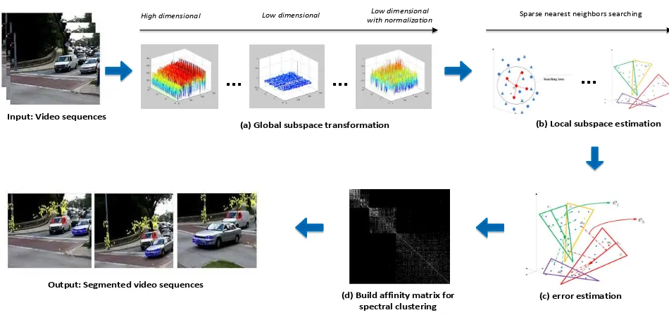
Input: Video sequences
...
...
High dimensional Low dimensional Low dimensional with normalization (d) Build affinity matrix for
spectral clustering Output: Segmented video sequences
Figure 2: Overview of the proposed framework.
4.1 Global Subspace Transformation
Due to the trajectory matrix of a rigid motion has a maximal rank 4, most people choose the projected dimension to bem= 4nor
5, wherenis the number of the motions in the video. Assume that the trajectory matrix isW2F×P, whereFis the number of frames
andPis the number of extracted trajectories. The traditional way to projectW2F×Pis Principal Component Analysis (PCA) (Abdi
and Williams, 2010), which can be formed as following,
z∗= max
zTz≤1z TΣz,
(5)
whereΣ =WTW is the covariance matrix ofW, solutionsz∗ represent the principal components. Usually, PCA can be ob-tained through performing singular value decomposition (SVD) forW. The solutionsz∗
are fully observed, which means they are constructed with all the input variables. However, if the prin-cipal componentsz∗
are built with only a few number of original variables but still can represent the original data matrix well, it should be easier to separate the underlying local subspaces from the transformed global subspace. The sparse PCA technique has been proved that it is robust to the noise and outliers in terms of dimensionality reduction and feature selection (Naikal et al., 2011), which aims to seek a low-dimensional sparse representa-tion for the original high-dimensional data matrix. In contrast to PCA, sparse PCA produces the sparse principal components that achieve the dimensional reduction with a small number of input variables but can interpret the main structure and significant in-formation of the original data matrix.
In order to contain the orthogonality of projected vectors in the global subspace, we apply the generalized power method for sparse PCA (Journ´ee et al., 2010) to transform the global subspace. Given the trajectory matrixW2F×P = [w1, ..., wF]T, where wf ∈
R2×P, f= 1, ..., Fcontains all the trackedP2-D feature points
in each framef. We can consider a direct single unit form as Eq. 6 to extract one sparse principal componentz∗
∈RP (Zou et al.,
2006, Journ´ee et al., 2010).
z∗(γ) = max
y∈BPzmax∈B2F(y
TW z)2
−γkzk0 (6)
whereydenotes a initial fixed data point from the unit Euclidean sphereBP = {y ∈ RP|yTy ≤ 1}, andγ > 0is the sparsity controlling parameter. If project dimension ism,1< m <2F, which means there are more than one sparse principal compo-nents needed to be extracted, in order to enforce the orthogonality for the projected principal vectors, (Journ´ee et al., 2010) extends Eq. 6 to block form with a trace function(Tr()), which can be defined as Eq. 7
controlling parameter vector, and parameter matrix
N =Diag(µ1, µ2, ..., µm)with setting distinct positive
diago-nal elements enforces the loading vectorsZ∗
to be more orthog-onal,Spm = {Y ∈ RP×m|YTY =Im}represents theStiefel manifold. Subsequently, Eq. 7 is completely decoupled in the columns ofZ∗(γ)
Obviously, the objective function in Eq. 8 is not convex, but the solutionZ∗γ
can be obtained after solving a convex problem in Eq. 9
(Journ´ee et al., 2010), a gradient scheme has been proposed to efficiently solve the convex problem in Eq. 9. Hence, the sparsity patternIfor the solutionZ∗is defined byY∗after Eq. 9 under the following criterion,
I=
active, (µjwiTyj∗)2> γj,
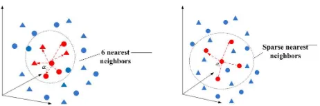
Figure 3: Illustration of 6-nearest neighbors and sparse nearest neighbors policy. The circles and triangles represent the data points from two different local subspaces respectively. The red points denote the estimated neighbors for the observed dataαi
from the same local subspace under the determinate searching area.
As a result, the seeking sparse loading vectorsZ∗ ∈ SP
m are
obtained after iteratively solving Eq. 9. After normalization, the global projected subspacefWm×P = normalize(Z∗)T is
achieved, which is embedded with multiple orthogonal underly-ing local subspaces.
4.2 Local Subspace Estimation
In order to cluster the different subspaces according to different moving bodies, the first step is finding out the multiple under-lying local subspaces from the global subspace. Generally, the estimation of different local subspaces can be addressed as the extraction of different data sets, which contain only the projected trajectories from the same subspace. One of the most traditional way is the local sampling (Yan and Pollefeys, 2006), which uses the KNN. Specifically, the underlying local subspace spanned by each projected data is found by collecting each projected data point and its corresponding K nearest neighbors, which are cal-culated by the distances (Yan and Pollefeys, 2006, Goh and Vidal, 2007). However, the local sampling can not ensure that all the ex-tracted K-nearest neighbors truly span one same subspace, which means an overestimation, especially for the video who contains a lot of degenerated/depended motions or missing data. Moreover, (Zappella et al., 2011) has testified that the selection of number K is quite sensitive, which depends on the rank estimation. In this paper, for the sake of avoiding the searching for only nearest neighbors and solving the overestimation problem we adopt the sparse nearest neighbors optimization to automatically find the set of the projected data points that span a same local subspace.
The assumption of sparse nearest neighbors is derived from SMCE (Elhamifar and Vidal, 2011), which can cluster the data point from a same manifold robustly. Given a random data pointxithat
draw from a manifoldMlwith dimensiondl, under the SMCE
assumption, we can find a relative set of pointsNi =xj, j6=i
fromMlbut contains only a small number of non-zero elements
that passes throughxi. This assumption can be mathematically
defined with Eq. 11
kci[x1−xi, ..., xP−xi]k2≤ǫ, s.t1Tci=1 (11)
wherecicontains only a few non-zero entries that denote the
in-dices of the data point that are the sparse neighbors ofxifrom the
same manifold,1Tci=1is the affine constraint andPrepresent
the number of all the points lie in the entire manifold.
We apply the sparse neighbors estimation to find the underlying local subspaces in our transformed global subspace. As shown in Fig. 3, with the 6-nearest neighbors estimation, there are four triangles have been selected to span the same local subspace with observed dataαi, because they are near toαithan the other
cir-cles. While, the sparse neighbors estimation is looking for only a
small number of data point that close toαi, in this way most of
the intersection area between the different local subspaces can be eliminated. In particular, we constraint the searching area of the sparse neighbors for each projected trajectory from the global subspace with calculating the normalized subspace inclu-sion (NSI) distances (da Silva and Costeira, 2009) between them. NSI can give us a robust measurement between the orthogonal projected vectors based on their geometrically consistent, which is formulated as
where the input is the projected trajectory matrix
f
Wm×P = [α1, ..., αP], andαiandαj, i, j= 1, ..., Prepresent
two different projected data. The reason of using NSI distances to constraint the sparse neighbors searching area is the geometric property of the projected global subspace. Nevertheless the data vectors which are very far away fromαidefinitely can not span
the same local subspace withαi. Moreover, in addition to save
computation times, the selection for the searching area with NSI distances is more flexible, which has a wide range of values, than tuning the fixed parameter K for nearest neighbors.
Furthermore, all the NSI distances are stacked into a vectorXi=
[N SIi1, ..., N SIiP]T, the assumption from SMCE in Eq. 11 can
be solved with a weighted sparseL1 optimization under affine
constraint, which is formulated as following
minkQicik1
s.tkXicik2≤ǫ,1Tci= 1
(13)
whereQiis a diagonal weight matrix and defined as
Qi = exp(exp(XP i/σ)
t6=iXit)/σ ∈ (0,1], σ > 0. The effect of the
positive-definite matrix Qi is encouraging the selection of the
closest points for the projected dataαiwith a small weight, which
means a lower penalty, but the points that are far away toαiwill
have a larger weight, which favours the zero entries in solution ci. We can use the same strategy as SMCE to solve the
opti-mization problem in Eq. 13 with Alternating direction method of multipliers (ADMM) (Boyd et al., 2011).
As a result, we can obtain the sparse solutionsCP×P = [c1, ..., cP]T
with a few number of non-zero elements that contain the infor-mations and connections between the projected data point and its estimated sparse neighborhoods. As investigated in SMCE (Elhamifar and Vidal, 2011), in order to build the affinity ma-trix with sparse solutionCP×P we can formulate a sparse weight
matrixΩP×P with vectorωi, which is built byωii = 0, ωij = cij/Xij
P
t6=icit/Xti, j 6= i. The achieved weight matrixΩP×P
con-tains only a few non-zero entries in column, which give the in-dices of all the estimated sparse neighbors and the distances be-tween them. Hence, we can collect each dataαiand its estimated
sparse neighborsNiinto one local subspaceSbiaccording to the
non-zero elements ofωi.
4.3 Error Estimation
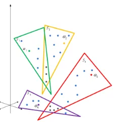
As illustrated in Figure 4, the local subspace estimation some-times leads to incorrect overlapping sparse neighbors. We pro-pose the following error function to resolve the overlapping esti-mation problem:
Figure 4: The geometrical illustration of incorrect local sub-space estimation with sparse neighbors. S1, S2, S3, S4 are
four estimated local subspaces spanned by the observed data α1, α2, α3, α4respectively.
b
βi, I ∈ Rm×mis an identity matrix. The geometrical
mean-ing of the error functioneit is the distance between the
esti-mated local subspace and projected data. As a consequence, after computing for each estimated local subspaceSbiits
correspond-ing error vectorei = [ei1,· · ·, eiP], we build an error matrix
eP×P = [e1,· · ·, eP], which contains the strong connection be-tween the projected data span a same local subspace.
In the end, we construct the affinity graphG= (V, E)with com-bining the estimated error matrixeP×P and the sparse matrix CP×P, whose the nodesV represent all the projected data points
and edgesEdenote the distances between them. In our affin-ity graph, the connection between each two nodesαiandαjis
determined by both theeijandωij. Therefore, the constructed
affinity graph contains only several connected elements, which are related to the data points span the same subspace, whereas there is no connection between the data points live in a differ-ent subspace. Subsequdiffer-ently, we perform the normalized spec-tral clustering (Von Luxburg, 2007) on the adjacent matrix of the affinity graph, and obtain the final clusters with different labels, and each cluster is related to one moving object.
5 EXPERIMENTAL RESULTS
Our proposed framework is evaluated on the Hopkins 155 dataset (Tron and Vidal, 2007) with comparing with state-of-the-art sub-space clustering and affinity-based motion segmentation algo-rithms.
Implementation DetailsMost popular subspace based motion segmentation methods (Elhamifar and Vidal, 2009, Yan and Polle-feys, 2006, Ma et al., 2007, Dragon et al., 2012, Ochs et al., 2014) have assumed that the number of motions has been already known. For the Hopkins 155 dataset, we give the exactly num-ber of clusters according to the numnum-ber of motions. In this work, the constrained area for searching the sparse neighbors is firstly varied in a range variables[10,20,30,50,100], then it turns out that the tuned constrained area performs equally well from 20 to 50, so we choose to set the number with 20, which accord-ing to the alternative number of sparse numbers. In our exper-iments, we have applied the PCA and sparse PCA for evaluat-ing the performance of our framework on estimatevaluat-ing the multiple local subspaces from a general global subspace with dimension m= 5. The sparsity controlling parameter for sparse PCA is set toγ = 0.01and the distinct parameter vector[µ1, ..., µm]is set
to[1/1,1/2, ...,1/m].
5.1 The Hopkins 155 dataset
The Hopkins 155 dataset (Tron and Vidal, 2007) contains 3 dif-ferent kinds sequences: checkerboard, traffic and articulated. For
each of them, the tracked feature trajectories are already been pro-vided in the ground truth and the missing features are removed as well, which means the trajectories in the Hopkins 155 dataset are fully observed and there is no missing data. We have computed the average and median misclassification error for comparison our method (O) with state-of-the-art methods: SSC (Elhamifar and Vidal, 2009), LSA (Yan and Pollefeys, 2006), ALC (Ma et al., 2007)and MSMC (Dragon et al., 2012), as shown in Table 1, Table 2, Table 3. Table 4 refers to the run times of our method comparing with two sparse optimization based methods: ALC and SSC. Obviously, as Table 1 and Table 2 show, the overall
er-Method ALC SSC MSMC LSA Opca Ospca
Articulated, 11 sequences
mean 10.70 0.62 2.38 4.10 2.67 0.55
median 0.95 0.00 0.00 0.00 0.00 0.00
Traffic, 31 sequences
mean 1.59 0.02 0.06 5.43 0.2 0.48
median 1.17 0.00 0.00 1.48 0.00 0.00
Checkerboard, 78 sequences
mean 1.55 1.12 3.62 2.57 1.69 0.56
median 0.29 0.00 0.00 0.27 0.00 0.00
All 120 sequences
mean 2.40 0.82 2.62 3.45 1.52 0.53
median 0.43 0.00 0.00 0.59 0.00 0.00
Table 1: Mean and median of the misclassification (%) on the Hopkins 155 dataset with 2 motions.
Method ALC SSC MSMC LSA Opca Ospca
Articulated, 2 sequences
mean 21.08 1.91 1.42 7.25 3.72 3.19
median 21.08 1.91 1.42 7.25 3.72 3.19
Traffic, 7 sequences
mean 7.75 0.58 0.16 25.07 0.19 0.72
median 0.49 0.00 0.00 5.47 0.00 0.19
Checkerboard, 26 sequences
mean 5.20 2.97 8.30 5.80 5.01 1.22
median 0.67 0.27 0.93 1.77 0.78 0.55
All 35 sequences
mean 6.69 2.45 3.29 9.73 2.97 1.94
median 0.67 0.20 0.78 2.33 1.50 1.30
Table 2: Mean and median of the misclassification (%) on the Hopkins 155 dataset with 3 motions.
Method ALC SSC MSMC LSA Opca Ospca
all 155 sequences
Mean 3.56 1.24 2.96 4.94 1.98 0.70
Median 0.50 0.00 0.90 0.75 0.00
Table 3: Mean and median of the misclassification (%) on all the Hopkins 155 dataset.
Method ALC SSC OP CA OSP CA
Run-time [s] 88831 14500 1066 1394
Table 4: Computation-Time (s) on all the Hopkins 155 dataset.
is one of the most accurate subspace-based algorithm. But due to the property of MSMC, which is based on computing the affini-ties between each pair trajectories, it is highly time-consuming. The checkerboard data is the most significant component for the entire Hopkins dataset, which in particular contains a lot of fea-tures points and many intersection problems between different motions. To be specific, the most accurate results for the checker-board sequences belong to our proposed framework with sparse PCA projection, either for two or three motions. It means that our method has the most accuracy for clustering different inter-sected motions. Table 3 shows our method achieves the least misclassification error for all the sequences from the Hopkins dataset in comparison with all the other algorithms. Although our method with sparse PCA or PCA projection is a bit loss of precision for the traffic sequences, we save a lot of computation times comparing with SSC and ALC as shown in Table 4. We evaluate our method with sparse PCA projection in comparison with LSA (Yan and Pollefeys, 2006), SSC (Elhamifar and Vidal, 2009), MSMC (Dragon et al., 2012), GPCA (Vidal et al., 2005), RANSAC (Fischler and Bolles, 1981) and MSMC (Dragon et al., 2012) in Figure 5 and Figure 6 on the Hopkins 155 dataset. Note that MSMC has not been evaluated on the checkboard sequence.
6 CONCLUSIONS
In this paper, we have proposed a subspace-based framework for segmenting multiple moving objects from a video sequence with integrating global and local sparse subspace optimization meth-ods. The sparse PCA performs a data projection from a high-dimensional subspace to a global subspace with sparse orthog-onal principal vectors. To avoid improperly choosing K-nearest neighbors and defend intersection between different local sub-spaces, we seek a sparse representation for the nearest neighbors in the global subspace for each data point that span a same local subspace. Moreover, we propose an error estimation to refine the local subspace estimation. The advantage of the proposed method is that we can apply two sparse optimizations and a simple error estimation to handle the incorrect local subspace estimation. The limitation of our work is the number of motions should be known firstly and only a constrained number of missing data can be han-dled accurately. The experiments on the Hopkins dataset show our method are comparable with state-of-the-art methods in terms of accuracy, and sometimes exceeds them on both precision and computation time.
ACKNOWLEDGEMENTS
The work is partially funded by DFG (German Research Founda-tion) YA 351/2-1. The authors gratefully acknowledge the sup-port.
REFERENCES
Abdi, H. and Williams, L. J., 2010. Principal component analysis. Wiley Interdisciplinary Reviews: Computational Statistics 2(4), pp. 433–459.
Boyd, S., Parikh, N., Chu, E., Peleato, B. and Eckstein, J., 2011. Distributed optimization and statistical learning via the alternat-ing direction method of multipliers. Foundations and Trends in Machine Learning 3(1), pp. 1–122.
da Silva, N. P. and Costeira, J. P., 2009. The normalized subspace inclusion: Robust clustering of motion subspaces. In: ICCV, pp. 1444–1450.
Dragon, R., Rosenhahn, B. and Ostermann, J., 2012. Multi-scale clustering of frame-to-frame correspondences for motion segmentation. In: ECCV, pp. 445–458.
Elhamifar, E. and Vidal, R., 2009. Sparse subspace clustering. In: CVPR, pp. 2790–2797.
Elhamifar, E. and Vidal, R., 2011. Sparse manifold clustering and embedding. In: NIPS, pp. 55–63.
Fischler, M. A. and Bolles, R. C., 1981. Random sample consen-sus: a paradigm for model fitting with applications to image anal-ysis and automated cartography. Communications of the ACM 24(6), pp. 381–395.
Goh, A. and Vidal, R., 2007. Segmenting motions of different types by unsupervised manifold clustering. In: CVPR, pp. 1–6.
Journ´ee, M., Nesterov, Y., Richt´arik, P. and Sepulchre, R., 2010. Generalized power method for sparse principal component anal-ysis. Journal of Machine Learning Research 11, pp. 517–553.
Kanatani, K., 2001. Motion segmentation by subspace separation and model selection. In: ICCV, pp. 586–591.
Ma, Y., Derksen, H., Hong, W. and Wright, J., 2007. Segmen-tation of multivariate mixed data via lossy data coding and com-pression. PAMI 29(9), pp. 1546–1562.
Naikal, N., Yang, A. Y. and Sastry, S. S., 2011. Informative fea-ture selection for object recognition via sparse pca. In: ICCV, pp. 818–825.
Ochs, P., Malik, J. and Brox, T., 2014. Segmentation of moving objects by long term video analysis. PAMI 36(6), pp. 1187–1200.
Tron, R. and Vidal, R., 2007. A benchmark for the comparison of 3-d motion segmentation algorithms. In: CVPR, pp. 1–8.
Vidal, R., Ma, Y. and Sastry, S., 2005. Generalized principal component analysis (gpca). PAMI 27(12), pp. 1945–1959.
Von Luxburg, U., 2007. A tutorial on spectral clustering. Statis-tics and computing 17(4), pp. 395–416.
Yan, J. and Pollefeys, M., 2006. A general framework for motion segmentation: Independent, articulated, rigid, non-rigid, degen-erate and non-degendegen-erate. In: ECCV, pp. 94–106.
Yang, M. Y. and Rosenhahn, B., 2014. Video segmentation with joint object and trajectory labeling. In: IEEE Winter Conference on Applications of Computer Vision, pp. 831–838.
Yang, M. Y., Feng, S. and Rosenhahn, B., 2014. Sparse opti-mization for motion segmentation. In: ACCV 2014 Workshops-Revised Selected Papers, pp. 375–389.
Zappella, L., Llad´o, X., Provenzi, E. and Salvi, J., 2011. En-hanced local subspace affinity for feature-based motion segmen-tation. Pattern Recognition 44(2), pp. 454–470.
(a)
(b)
(c)
(d)
(e)
(f)
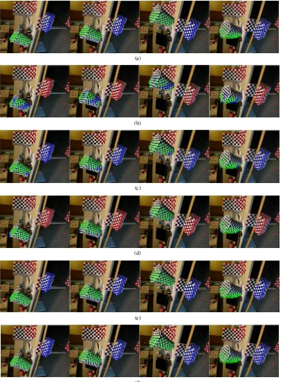
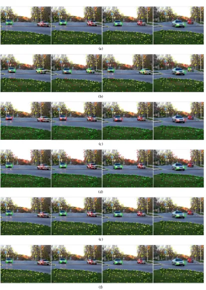
Figure 5: Comparison of Our approach with ground truth and the other approaches on the1RT2RCvideo: 5(a): GroudTruth; 5(b): GPCA, error: 44.98%; 5(c): LSA, error:1.94%; 5(d): RANSAC, error: 33.66%; 5(e): SSC, 0%; 5(f): Our, 0%on the1RT2TC
(a)
(b)
(c)
(d)
(e)
(f)