www.elsevier.comrlocateratmos
A method for the parameterization of cloud optical
properties in bulk and bin microphysical models.
Implications for arctic cloudy boundary layers
Jerry Y. Harrington
a,), Peter Q. Olsson
ba
Department of Meteorology, The PennsylÕania State UniÕersity, UniÕersity Park, PA 16802 USA b
Alaska Experimental Forecast Facility, UniÕersity of Alaska Anchorage, Anchorage, AK, USA
Received 16 March 2000; received in revised form 5 October 2000; accepted 27 October 2000
Abstract
Computationally efficient and numerically accurate methods for computing band-averaged cloud optical properties for radiative transfer interactions with various microphysical parameteriza-tions are described. Parameterizaparameteriza-tions for bulk microphysical models employing generalized gamma distribution representations of the size spectra and binned representations, in which the size spectra fluctuate with time, are discussed. It is shown that simple exponential fits and look-up tables may be used with minimal computational cost and high accuracy for bulk microphysical models. Binned microphysical representations may be parameterized using mean properties for each bin, if averaged appropriately.
The implications for the radiative scheme are discussed in comparison with the computed
Ž .
radiative budget of fallrspring season mixed-phase Arctic stratus clouds ASC . Compared to liquid clouds of the same water path, mixed-phase ASC absorb and reflect less radiation, and
Ž .
transmit more radiation to the surface. This results in greater cooling warming of the surface, by
y2 Ž .
up to 60 W m , in the infrared solar by mixed-phase clouds. The radiative properties of mixed-phase clouds show a significant sensitivity to crystal habit for clouds with ice water paths
R25 g my2. Surface net fluxes and cloud absorption may vary by up to 15 W my2, depending on
the ice habit. It is also shown that mixed-phase clouds are more sensitive to the choice of ice
Ž .
effective radius re,i than liquid clouds are to r . Using values of from the literature, it is showne that the surface net fluxes can vary by as much as 50 W my2
depending on the value of r .e,i
Ž .
Furthermore, it is shown that the sign of the surface net flux i.e. warming or cooling may be dependent on the value of re,i selected.q2001 Elsevier Science B.V. All rights reserved.
Keywords: Arctic stratus; Radiation budget; Ice optical properties; Mixed phase
)Corresponding author. Tel.:q1-814-863-1584; fax:q1-814-865-3663.
Ž .
E-mail address: [email protected] J.Y. Harrington .
0169-8095r01r$ - see front matterq2001 Elsevier Science B.V. All rights reserved.
Ž .
1. Introduction
Increasingly, atmospheric models are incorporating more complex and physically realistic microphysical models within their frameworks. These schemes vary in their
complexity from the number of moments of the droprice spectra predicted to the
number of classes of hydrometeors defined. At the same time, accurate and efficient computations of the atmospheric radiative budget are necessary for reasons ranging from
Ž .
climate considerations e.g., Curry and Ebert, 1990; Royer et al., 1990; Curry, 1995 to
Ž . Ž
the detailed simulation of clouds on the Large Eddy Simulation LES scale e.g.,
.
Stevens et al., 1996 . Since real clouds interact strongly with both solar and infrared radiation, it is desirable for current radiation schemes to interact realistically with the clouds predicted in these models.
Microphysical schemes that are coupled to dynamical models can generally be divided into two classes: the first is normally referred to as a bulk or explicit
Ž .
microphysical scheme e.g., Walko et al., 1995 and the second is that of a binned
Ž .
microphysical scheme e.g., Feingold et al., 1994 . Bulk microphysical schemes vary in complexity. However, they are all built upon the same underlying assumption, which fixes the functional form of the hydrometeor size spectra. In many cases, this functional
Ž .
form is assumed to be the generalized gamma distribution function Walko et al., 1995 . Using this function, either one or two moments of the hydrometeor spectra are
Ž .
prognosed. In most cases, one-moment schemes predict the total mass mixing-ratio rl
Ž .
of a given hydrometeor class e.g., Rutledge and Hobbs, 1984; Walko et al., 1995 while
Ž
two-moment schemes also predict the number concentration e.g., Ferrier, 1994; Meyers
.
et al., 1997 . The number of hydrometeor classes used in a model is somewhat dependent upon the class distinctions made by the developer; however, most follow a
Ž .
similar construction e.g., Ferrier, 1994; Walko et al., 1995; Meyers et al., 1997 . Binned microphysical models make no assumptions about the functional form of the hydrometeor size spectrum. Instead, a preset number of bins are defined for each hydrometeor class and the number concentration and mass are then predicted for each
Ž .
bin Feingold et al., 1994; Kogan et al., 1995; Reisin et al., 1996 . Such models allow for a much more realistic evolution of the hydrometeor spectra, but at a high computa-tional cost.
In each of these modeling frameworks, assumptions must be made about the shape and growth characteristics of the various ice species that exist within the model. A successful radiative transfer scheme should include appropriate parameterizations of the cloud optical properties for each hydrometeor class, whether water or ice.
The purpose of the present paper is twofold. First, we present the cloud microphysi-cal-radiative transfer coupling developed for use in the Regional Atmospheric Modeling
Ž .
System RAMS . We illustrate the parameterization’s flexibility and its potential accu-racy. Second, we use this parameterization to examine the importance of various microphysical parameter choices to the computation of the radiative heat budget of the
Ž .
mixed-phase Arctic cloudy boundary layer BL and the surface. Few studies have examined the radiative influence of mixed-phase clouds in general, and those that have
Ž .
ŽSun and Shine, 1994 and may even have a significant impact on climate Sun and. Ž .
Shine, 1995 . Mixed-phase clouds cover the Arctic Ocean throughout a large portion of
Ž .
the year e.g., Intrieri et al., 1999 and, thus, have a significant impact on the radiative
Ž
budget of the Arctic Ocean. This is quite important as many studies e.g., Curry and
.
Ebert, 1990; Royer et al., 1990; Curry, 1995; Lynch et al., 1995 have illustrated the possible sensitivity of the Arctic system to alterations in cloud radiative properties,
Ž .
particularly the frequently observed low-lying Arctic stratus clouds ASC . Since
microphysical data are sparse for ASC, we use microphysical information derived from
Ž .
RAMS bin microphysical simulations of ASC Harrington et al., 1999 , which compare favorably with observations in our radiative computations. We pick cases that span a large range of liquid and ice water paths, covering the ranges observed in the Arctic. This model information is useful since the simulated clouds behave like observed ASC and have microphysical structures similar to available observations. However, it must always be kept in mind that this information is derived from a numerical model. Thus,
our results should be viewed as an attempt to assess the possible qualitatiÕe impacts of
cloud microstructure on the Arctic radiation budget.
2. Bulk model parameterization
Modeling frameworks such as RAMS are computationally intensive and require radiation routines that are efficient yet accurate. For this reason, two-stream radiation models are frequently used. The coupling of any two-stream radiative transfer scheme to a microphysical model requires the efficient computation of cloud optical properties.
Ž . Ž .
These consist of the single scatter albedo v , the optical depth t , and the asymmetry
Ž .
parameter g . These parameters are computed for each band of the radiative transfer model and are combined from values computed for each hydrometeor type. Our current RAMS radiation model has two band structures: a broader band structure which is based
Ž . Ž .
on Ritter and Geleyn 1992 RG; three solar and five infrared bands and a narrower
Ž . Ž .
band structure based on Fu and Liou 1992 FL; six solar and 12 infrared bands . This
Ž . Ž .
model is fully described in Harrington 1997 and briefly in Harrington et al. 1999 . Bulk microphysical models in use today predict the evolution of a variety of hydrometeor classes and various moments of the distribution function. RAMS predicts the evolution of seven separate hydrometeor species: cloud droplets, rain, pristine ice,
Ž .
snow, aggregates, graupel, and hail Walko et al., 1995; Meyers et al., 1997 . Each class is defined by particular growth mechanisms, and not necessarily by standard
terminol-Ž .
ogy for details see Walko et al., 1995 .
Ž
In RAMS and in several other microphysical modeling frameworks e.g., Ferrier,
.
1994; Mitchell, 1994 , hydrometeors are assumed to have the form of gamma distribu-tion,
ny1
Nt D 1 D
n D
Ž .
sž /
y expž /
y ,Ž .
1where N is the number concentration,t G is the gamma function, n is a parameter describing the shape of the size spectrum, D is the diameter of the hydrometeors, and
Dn is the characteristic diameter of the distribution. For ice hydrometeors, which
typically lack spherical symmetry, D and D are replaced respectively by L and L ,n n
where L is defined as the maximum dimension of a given crystal habit.
This functional form has many desirable attributes. It is easily integrated and frequently it can be fit to observed spectra. Furthermore, its variables have clear physical interpretations; the mean size of hydrometeors of a gamma distribution is given by DsnD . The shape parameter,n n, describes the spectral breadth of the distribution. A
value of ns1 produces a broad, exponential distribution function while a larger value
Ž .
of n say 15 produces a very narrow spectrum.
2.1. Bulk optical properties: liquid and ice
A major difficulty with computing the optical properties for microphysical models is
Ž .
that one must integrate not only over the size distribution, n D , but also over a given
Ž . Ž .
radiative band-width Dl. Thus, for the extinction Qext the following integral must be
Ž .
solved Slingo and Schrecker, 1982 ,
`
bexts
H H
A D QŽ .
extŽ
D, ml. Ž .
n D d D E dl lrH
E dl l,Dl 0 Dl
ElsSl
Ž
Solar ,.
ElsBŽ
l, Ts. Ž
Infrared ,.
Ž .
2Ž .
where A D is the cross-sectional area of any hydrometeor, m is the complex index of
refraction, E is the solarl rinfrared energy density, and Tss273 K is the reference value
Ž .
used for the Planck function. Eq. 2 is known as thin averaging, which works quite well
for extinction but tends to underestimate v in broad-band models. In order to reduce
this over-absorption, the thick averaging of Edwards and Slingo, 1996 is used to
determine the band-averaged v,
where r is the reflectance of an infinitely thick layer see Edwards and Slingo, 1996 ,`
Ž .
and r` and g are averaged similarly to Qext in Eq. 2 . We use thick averaging for
liquid drops and thin averaging for ice crystals as this produces excellent broad-band
Ž .
accuracy in comparison to a 220 band model Edwards and Slingo, 1996 .
2.1.1. Liquid phase
Ž .
is Anomalous Diffraction Theory ADT , but this theory can produce relatively large
Ž . Ž .
errors Mitchell, 2000 . Fortunately, Mitchell 2000 has derived a method which vastly
Ž .
improves ADT the Modified ADT, or MADT by parameterizing the ‘‘missing
physics’’ associated with internal reflectionrrefraction, resonance tunneling, and edge
effects that are not accounted for in ADT. We derive the optical properties of water
Ž
drops with this theory since the errors associated with it are quite small see Mitchell,
.
2000 .
Modified ADT, like ADT, gives the extinction and absorption coefficients of spherical drops. The ADT optical properties are modified in the following manner in
Ž .
MADT see Appendix A for definitions ,
Cres
Qext , m
Ž
D,l, m.
sž
1q/
QextqQedge,Ž .
42
Qabs , m
Ž
D,l, m.
sŽ
1qCirqCres.
Qabs,Ž .
5where Qext and Qabs are the ADT extinction and absorption coefficients, Cres is the
modification for resonance tunneling, Cir is the modification for internal reflectionr
re-fraction, and Qedge is the modification for edge effects. These functions allow the
Ž . Ž .
integral over the size distribution in Eq. 2 to be evaluated analytically. Mitchell 2000 has already solved this problem for a form of the gamma distribution function. However, with a view to putting this solution in a form usable in RAMS, we have solved the
Ž .
integral for the generalized gamma distribution given by Eq. 1 . The extinction and
absorption integrated over size, defined respectively as bext and babs, become,
bextsA QextqQres ,eqQedge ,
Ž .
6babssA QabsqQirqQres ,
Ž .
7where A is the integrated cross-sectional area of the distribution, and the other terms are the integrated ADT extinction and absorption, and the integrated MADT correction
Ž .
terms see Appendix A . The above solution explicitly shows the impact of each additional term in MADT on the total extinction and absorption, and is more succinct
Ž .
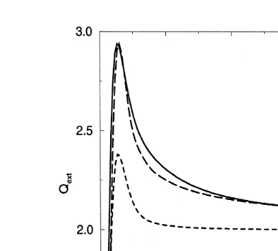
than the solution given in Mitchell 2000 . These functions are easily coded and require little computation time compared to an approach based on Lorenz–Mie theory. When integrated over a radiation model bandwidth, errors are reduced even further. As an example, Fig. 1 shows a comparison between MADT, ADT and Lorenz–Mie theory for
Qext as a function of D . The extinction shows only small errors near characteristicn
diameters of about 10mm.
While MADT gives a fairly accurate representation of Qext and v, it does not give
information about the asymmetry parameter. Because of the time-consuming
computa-tions involved, a dataset was constructed of values for one distribution shape,ns6, for
Fig. 1. Computations of Qext using MADT, Lorenz–Mie theory, and ADT for the 8.3–9.0mm band of the radiation model.
2.1.2. Ice phase
Since ice crystals have edges, the accurate computation of ice crystal optical properties is not as straight-forward as it is for liquid drops. Many methods exist for ice optical property computations with perhaps the simplest being the use of equivalent surface area or volume spheres. However, such methods may not be appropriate
ŽGrenfell and Warren, 1999; Mitchell and Arnott, 1994; Stackhouse and Stephens, 1991;
. Ž .
Wielicki et al., 1990 . For example, Stackhouse and Stephens 1991 found that the measured albedo of cirrus clouds was significantly larger than that predicted with ice
Ž
spheres. Ray-tracing results and the parameterizations based on them e.g., Takano and
.
Liou, 1989; Fu and Liou, 1992; Ebert and Curry, 1992 have shown that ice crystals scatter more and absorb less than equivalent volume spheres. This result has led to
Ž .
successful methods like Grenfell and Warren’s 1999 in which each crystal is modeled as a collection of spheres that have the same total volume and surface area as a single crystal. Even though more successful scattering methods are being developed for ice
Ž . Ž .
crystals, the work of Doutriaux-Boucher et al. 2000 and Labonnote et al. 2000 cast doubt on the use of pure-ice hexagonal crystals for the characterization of ice cloud optical properties. In their studies of cirrus clouds, the best retrievals were obtained using hexagonal ice crystals with inhomogeneous inclusions of air bubbles. Even though this is the case, it is difficult to know in advance the percentage of air inclusions in a population of crystals and, therefore, we ignore this factor in our studies. In addition, most of the above approaches for calculating ice cloud optical properties are tied to particular band structures and ice classes while the method of Grenfell and Warren
Ž1999 is roughly similar to our method, which is described below..
Ž .
We use the approach described in Mitchell and Arnott 1994 and Mitchell et al.
ADT for ice hydrometeors versatile enough to be implemented in a variety of micro-physical frameworks. Additionally, this technique compares well to ray-tracing results. In this method, the ADT absorption for large spheres is modified by including the
Ž .
internal reflectionrrefraction term Cir and by replacing the distance that a ray passes
Ž .
through a sphere with the effective distance de that a ray passes through an ice crystal.
This gives,
4pni
Qabs ,is 1qCir
Ž
de.
1yexpž
y de/
,Ž .
8l
Ž . Ž .
where Cir is defined in Eq. A4 . We use formulae from Mitchell and Arnott 1994 ,
Ž . Ž .
Mitchell et al. 1990 , and Auer and Veal 1970 to compute values of d for three icee
classes: hexagonal plates, hexagonal columns, and five-branch bullet rosettes. Fig. 2
Ž .
shows d as a function of the maximum dimension of the crystal L . As expected, thee
effective distance is much shorter for non-spherical ice than for spheres and this reduces the absorption by crystals.
Ž .
In order to integrate Eq. 8 analytically over the size distribution, we follow Mitchell
Ž .
and Arnott 1994 and fit d as a linear function of L. Since d is obviously non-lineare e
in L, we use linear fits over the following five ranges of L: 1–30, 30–100, 100–500,
500–2000, and 2000–10000mm. Such a breakdown produces excellent accuracy in the
Ž . Ž .
fits to within 5% but requires the integral over size in Eq. 2 to be evaluated over a set of truncated size ranges,
Lh
babs ,i
Ž
L , Ll h.
sH
P L QŽ .
abs ,iŽ
L, m,l. Ž .
n L d L,Ž .
9Ll
where L and Ll h are the lower and upper limits defined by the piece-wise linear
Ž .
endpoints, and P L is the projected crystal area that is parameterized as in Mitchell and
Ž .
Fig. 2. Comparison of de for various ice habits. Included in the figures are spheres dash-dotted line ,
Ž . Ž . Ž .
Ž . Ž .
Arnott 1994 . We recast the form of the solution given in Mitchell et al. 1996 for the generalized gamma distribution as,
babs ,i
Ž
L , Ll h.
sP L , LŽ
l h.
Qabs ,iŽ
L , Ll h.
yCirŽ
L , Ll h.
,Ž .
10where the limits of integration are explicitly shown. The three terms above show the dependence of the absorption on the average projected area, the ADT absorption
coefficient, and the internal reflectionrrefraction term, all of which are given in
Appendix A.4. The total absorption is then determined by summing the integral
solutions for the five d size-ranges,e
5
babs ,is
Ý
babs ,iŽ
Ll , j, Lh , j.
.Ž .
11js1
Ž .
For extinction, we use equivalent d spheres as in Mitchell et al. 1996 , except thate
Ž .
we use MADT instead of ADT to compute. Mitchell et al. 1996 compute the mass and
number median sizes for equivalent d sphere distributions. These sizes are used toe
derive new N, D , andn n for use in the extinction computations. Instead of following
this approach, which can lead to numerical problems for very narrow distributions
ŽHarrington, 1997 , we hold the total mass, number, and. n constant, and derive a new
Ž . Ž
characteristic size Dn,s for the equivalent de sphere distribution see Harrington,
. Ž .
1997 . This value of Dn,s is then used in Eq. 6 to compute the total extinction at a
particular wavelength. Numerical tests show that this procedure produces the same
Ž .
values as the method of Mitchell et al. 1996 , but requires fewer transformations. Since little information is available regarding the asymmetry parameter for crystals at
infrared wavelengths, we calculate g using spheres with sizes equal to d for a given icee
crystal. This technique reduces g as compared to equivalent volume spheres, which is
Ž
desirable as g for spheres is uniformly larger than it is for crystals Takano and Liou,
.
1989; Grenfell and Warren, 1999 . These computations also compare well with the
Ž .
reduced-g method of Sun and Shine 1994 . Additionally, since g variation has a small influence on diabatic processes, this should be a tollerable approximation.
This method, coupled with thin averaging, is used to derive the band-averaged optical
properties for the three ice habits. Fig. 3 shows v for columns, plates, and bullet rosette
crystals for the 8.33–9.0mm band of the radiation model. In comparison with equivalent
volume spheres, the reduced effective distance leads to greater scattering and less
Ž . Ž .
Fig. 4. Comparison between computations of Qextand vusing MADT points and fits solid lines for bands
Ž .
Ž .
absorption by the crystals. As shown by Mitchell et al. 1996 , on the cloud scale this leads to comparatively more reflection and less absorption.
2.1.3. General parameterization
Even though the above methods are computationally expedient, the integral over
Ž .
radiation band-width is still too costly to compute repeatedly at run-time. Thus, Eq. 2 needs to be parameterized in some way. This is accomplished by fitting the optical
Ž .
property computations for each band over the effective radius re with an
exponential-sum fit,
s sa qa eb1reqa eb2re,
Ž .
12opt 0 1 2
where sopt stands for either Qext, v, or g. Fig. 4 shows fits of Qext and v for three
bands of the RG radiation band-structure. These bands were chosen as examples because
they span the simplest and most difficult curve fits. A distribution shape of ns6 was
Ž .
used for these computations and is characteristic of a weakly drizzling liquid-only
Ž .
ASC Olsson et al., 1998 . Note the accuracy of the fits, particularly at small r wheree
the curves are highly non-linear. Errors never exceed 4% for any of the fits. Similar
Ž .
accuracy was obtained for the asymmetry parameter g , and for the optical properties of ice crystals.
It should be noted that the decision to fit the optical properties as a function of r ise
made with some foresight. As discussed above, all bulk microphysical models require an
Ž .
a priori choice for the shape of the size spectrum i.e.n for a gamma distribution . Thus,
the numerical fits must be recreated anytime n is changed. This is not a difficulty for
Ž .
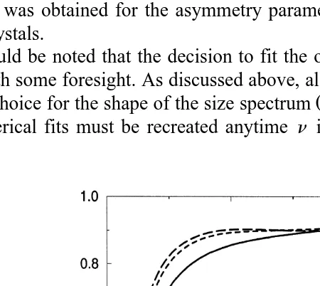
Fig. 5. Asymmetry parameter plotted as a function of r for different distribution shapes,e ns2 solid line , 6
Qext or v as these fits can be quickly recomputed. However, this is a problem for the computation of g, which requires the use of Lorenz–Mie theory.
Ž .
We circumvent this problem by adopting the approach of Hu and Stamnes 1993 .
This work showed that when optical properties for varying n were plotted against r ,e
the resultant curves were fairly independent of n. This result is found to hold in Fig. 5
and suggests that one can compute the optical properties as functions of r for a givene n
and then use that information for any gamma distribution.
Ž .
Of course, there are errors associated with this method when size;l . For example,
solar bands show the greatest errors at small r , below those typically observed ine
Ž
clouds. However, errors of the same magnitude occur in the infrared near res10 not
. Ž .
shown , which is within the range typical of marine stratocumulus Stephens, 1978 .
Since g has a smaller influence on diabatic processes than Qext or v, this error should
be tolerable. In fact, calculations using this method for ASC with differing n are only
slightly affected by using this method for computing g.
3. Bin model parameterization
Bin microphysical models in use today vary in their complexity and structural details
Že.g., Feingold et al., 1994; Kogan et al., 1995 . The liquid-phase bin microphysical.
Ž .
scheme used in the RAMS model is essentially that of Feingold et al. 1994 as modified
Ž .
by Stevens et al. 1996 while the mixed-phase bin microphysics is that of Reisin et al.
Ž1996 . For both schemes condensation deposition , evaporation sublimation , and. Ž . Ž .
collision–coalescence are solved on a discrete grid using the method-of-moments
ŽTzivion et al., 1989; Stevens et al., 1996 . In our work, the grid is defined by size.
boundaries covering the space from 3.125 to 1008mm. These diameter boundaries are
defined by mass-doubling between bin edges where edge kq1 is related to edge k by
mkq1s2 m . This translates into the following formula for the diameter edges, Dk ks
2Žky1.r3D , where D is 3.125 mm. A definition of this parameter space requires
1 1
Ž . Ž . Ž .
specification of 25 bins 26 edges with both number concentration Nk and mass Mk
for each bin varying in both time and space. To most accurately represent cloud optical properties, the radiative transfer model should make use of the bin information as it evolves.
3.1. Bin optical properties
With a bin microphysical representation, the size spectrum can vary significantly
Ž .
during a model run. While it is possible to use the method of Hu and Stamnes 1993 for bin models, there exists a more accurate method of computing the optical properties from the bin microphysical model information during model integration that is still computationally expedient. Additionally, this approach is necessary for coupling
radia-Ž
tion into the vapor growth equations in bin models see Harrington et al., 2000; Wu et
.
Ž .
In order to use Eq. 2 , the continuous integral over size must now be broken into a discrete sum over individual bins and be formulated as a function of the mean diameter
ŽDk.of each bin. However, since the mean diameter in each bin varies with time, and
since the wavelength and size dependence are intimately connected through
Ž .
Qext D , m,k l, Nbins
bexts
H
ElÝ
A DŽ .
k QextŽ
D , m,k l.
N dk lrH
E dl l,Ž .
13Dl ks1 Dl
is not efficient to solve during model integration. Again, this is because the wavelength integral must be numerically computed.
Ž .
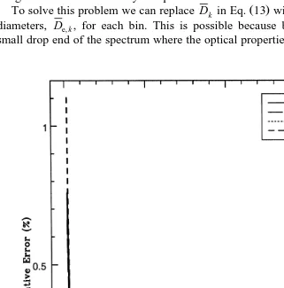
To solve this problem we can replace D in Eq. 13 with the average of the bin edgek
diameters, D , for each bin. This is possible because bin resolution is finest at thee, k
small drop end of the spectrum where the optical properties vary the most. By using this
Fig. 6. Relative errors associated with the bin optical property method for 4.6–8.3mm band. Errors for the
Ž .
method, the integral over wavelength may be computed before-hand since the De, k are fixed in time. Thus, the above integral is approximated as,
Nbins
Similar forms are easily derived forvand g by thin and thick averaging. For all optical
Ž .
properties, solutions to Eq. 15 are computed and stored as model input. During RAMS
Ž .
integration, Eq. 14 is used to compute the optical properties of drops and ice crystals. To test the accuracy of this method, computations were done using gamma distribu-tion funcdistribu-tions for which accurate analytical soludistribu-tions are known. Tests were then
conducted by breaking a gamma distribution of a given shape, ns6, into 25 discrete
bins and then applying the above method to compute the optical properties. Fig. 6 shows the relative error associated with using the bin method to derive the optical properties
Ž .
for a range of distribution mean sizes 1 to 400mm and for a particular radiation band.
Note that errors in the bin method are, in general, quite small. In particular, the bin method over-estimates the optical properties by about 1% for extremely narrow
distribu-Ž .
tions Dmean;1 . For distributions with DmeanR4 errors are negligible. This was also
found to be true for the ice-phase parameterization.
4. Radiative impacts of ASC
In order to illustrate the flexibility of the above scheme and the importance of microphysical characterization of mixed-phase ASC as regards the radiative heat budget, we have conducted a set of studies using microphysical output from previous modeling
Ž .
efforts. This allows us to illustrate two things: 1 the influence of the choice of
Ž .
microphysical characterization and structure on the radiative heating, and 2 the
influence of the ice phase on the cloud radiative properties. All of the following
Ž .
computations are done for solar zenith angles u0 F608 and with a surface albedo of
Ž .
0.65 Curry, 1986 , except where noted.
The cases used in this study are the mixed-phase ASC cases described in Harrington
Ž . Ž
et al. 1999 . Our discussions are limited to the diabatic heatingrcooling i.e. absorption
.
and emission by the cloud layer and the net surface fluxes for two reasons. First of all,
radiative heatingrcooling significantly influences the dynamics and, hence, the
evolu-Ž .
tion of ASC see Olsson et al., 1998; Harrington et al., 1999; Jiang et al., 2000 .
Alterations in cloud microstructure lead to changes in the radiative heatingrcooling of
Ž
the cloud layer, which then alters the dynamics and thickness of the cloud layer Boers
. Ž . Ž . Ž .
Ž .
give us some idea of how much the boundary layer BL is warming or cooling due to the radiative properties of a given cloud.
Ž
Second, since ASC are quite ubiquitous e.g. Herman and Goody, 1976; Utall et al.,
.
1999; Intrieri et al., 1999 , they have a significant influence on the Arctic surface
Ž . Ž .
radiation budget Curry, 1995 and, thus, the sea ice thickness Curry and Ebert, 1990 . In fact, it has been suggested that alterations in cloud microphysical properties can lead
Ž .
to as much as a 3-m alteration of the average sea-ice thickness Curry and Ebert, 1990 .
Ž .
In addition, Royer et al. 1990 have shown that alterations in sea-ice coverage can provide a feedback to the cloud coverage in either a positive or a negative fashion
Ždepending on the cloud parameterization. such that the sea ice either grows or
disappears. Hence, we examine how important the characterization of cloud
microstruc-Ž y q.
ture might be to the prediction of the surface net flux FnetsF yF . These
parameters, while not exhaustive, are sufficient to illustrate the potential impacts of cloud microstructure on the radiative heat budget of the cloudy BL and the surface.
4.1. Selected cases
Model output archived during the simulated evolution of mixed-phase ASC described
Ž .
in Harrington et al. 1999 is used selectively in this study. Particular time periods in the
Ž .
cloud evolution have been chosen, which have: 1 thick liquid cloud structure with
Ž . Ž .
some ice precipitation, 2 thin liquid cloud with a large amount of ice, and 3 thin cloud composed almost equally of ice and liquid. Since these runs were done with the
Ž .
bin-resolving microphysics of Reisin et al. 1996 , detailed liquid and ice crystal
distributions are available at each grid-point. The model output for each of these cases contains 61 columns of microphysical information. Since each model column is treated independently by the radiation model, the radiative analysis covers a broad range of
Ž y2. Ž y2.
liquid water paths LWP ;6–120 g m and ice water paths IWP ;6–80 g m .
Ž
These ranges of LWP and IWP cover those observed in Arctic Stratus Curry et al.,
.
1996; Hobbs and Rangno, 1998 , and the simulated clouds compare well with
observa-Ž .
tions Harrington et al., 1999 . Thus, this information forms a surrogate data set suitable
Ž .
for radiative analysis this procedure is similar to the approach of Duda et al., 1996 .
Ž . Ž .
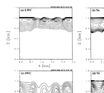
Fig. 7a–d shows the liquid water content LWC , drop concentration N , ice waterc
Ž . Ž .
content IWC , and ice concentration Ni for hour 6 of the control case described in
Ž .
Harrington et al. 1999 . This case, which we will call the thick liquid ASC or TLA, has
Ž .
a significant amount of LWC for the arctic environment spread through approximately
Ž y3.
a 300-m depth. Drop concentrations are fairly small Q14 cm due to the Bergeron–
Ž
Findeisen process that causes many of the small drops to evaporate Harrington et al.,
.
1999 . The simulated cloud produced weak ice precipitation from the liquid layer as the
Ž y1. Ž y1.
ice concentrations at these temperatures T;y8 l are small NiQ0.18 l . This
field is a characteristic snapshot of the evolution of this mixed-phase cloud layer, which continually precipitated small amounts of ice. Such cloud evolution is similar to
Ž .
previously observed cases e.g. Pinto, 1998; Hobbs and Rangno, 1998 and to observed
Ž .
arctic clouds over the SHEBA site Intrieri et al., 1999; Curry et al., 2000 .
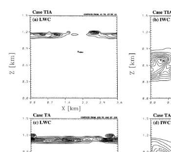
The second and third cases used are shown in Fig. 8. The first is a thick ice ASC
Ž . Ž . y3 Ž . y3 Ž . y3 Ž .
Fig. 7. Case 5CTRL at 6 h TLA . Panels: a LWC in g m , b N in cmc , c IWC in g m , and d Ni
in ly1
.
relatively large amount of ice below. This case is from a period of rapid glaciation
Ž .
described in Harrington et al. 1999 . Liquid water contents are never greater than 0.07 g
my3; however, IWCs become as large as 0.15 g my3. While this IWC may seem
somewhat large for the arctic, mixed-phase clouds with IWC values as high, and greater,
Ž
have been observed during the transition seasons e.g. Curry et al., 2000; Olsson and
.
Harrington, 2000 .
Ž .
The third case is a thin ASC TA, Fig. 8c and d and is characterized by a very thin
Ž y3.
upper liquid layer LWCF0.045 g m and a deep, but optically thin lower ice layer
ŽIWCFF0.028 g my3.. Such thin layers occurred in our numerical simulations
between periods of glaciation. This tenuous ice layer is similar to the clear-sky ice
Ž .
crystal precipitation cases frequently observed in the Arctic see Curry et al., 1996 ,
Ž .
though the temperature T;y148C is warmer here. Some cases from SHEBA exhibit
Ž .
such a structure Curry et al., 2000 .
Ž . Ž . Ž . y3 Ž .
Fig. 8. Thick mixed-phase TIA and thin mixed-phase TA clouds. Panels: a LWC in g m , b IWC in g
y3 Ž . y3 Ž . y3
m , c LWC in g m , and d IWC in g m .
selected cases, using optical properties that correspond exactly to what is predicted by the microphysical model. Second, sensitivity studies are conducted to determine how
Ž .
important ice crystal habit and ice effective radius re,i might be to the radiative heat
budget of the cloud layer and surface.
Table 1
Summary of bin model simulations used as surrogate data for the radiative computations Simulation Acronym Description
y3 Ž
Thick liquid ASC TLA 300-m-thick liquid cloud, small amount of ice LWCQ0.25 g m ,
y3.
IWCQ0.06 g m
y3 Ž
Thick ice ASC TIA Thick ice layer topped with very thin liquid cloud LWCQ0.07 g m ,
y3.
IWCQ0.15 g m
Thin ASC TA Optically thin liquid layer overlying deep, but optically thin ice layer
y3 y3
4.2. RadiatiÕe properties of the selected cases
In this section, we present radiative calculations using bin-microphysical output from RAMS in conjunction with the bin optical properties scheme discussed above. Our intent
Ž .
here is to illustrate the potential influence of various mixed-phase liquid-ice combina-tions on the radiative budget. Since the model simulacombina-tions assumed plate crystals, these are also assumed in the optical properties. Calculations presented below are for a solar
Ž .
zenith angle u0 of 608. The influence of u0 variation is discussed in later sections.
Ž . Ž .
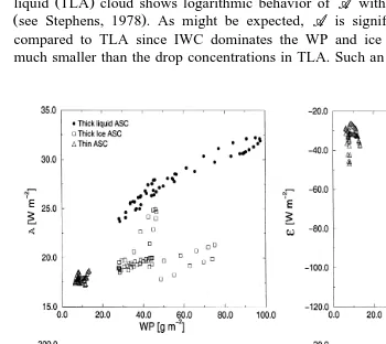
Fig. 9 shows the solar absorption AA and the total IR cooling of the cloud ´ , along
Ž . Ž .
with the net surface solar Fnet,sw and infrared Fnet,lw fluxes spanning the range of
Ž .
simulated water paths WPsLWPqIWP for all three cases. The case of the mostly
Ž .
liquid TLA cloud shows logarithmic behavior of AA with WP, which is well-known
Žsee Stephens, 1978 . As might be expected,. AA is significantly reduced in TIA as
compared to TLA since IWC dominates the WP and ice particle concentrations are much smaller than the drop concentrations in TLA. Such an effect has also been shown
Ž . Ž . Ž . Ž .
Ž .
by Sun and Shine 1994 . Additionally AAdoes not vary much with WP and is, in fact,
fairly constant. There are two reasons for this behavior. First, ice concentrations are low
Ž y1.
in these clouds typically Q10 l allowing for high transmission. Second, as IWP
increases, N generally decreases due the process of ice aggregation. Because N isi i
decreasing with IWP, AA is not as large as might be expected when conserving WP
alone. Note also that for TIA a few of the points tend toward the solutions for the predominantly liquid cloud. This is due to the fact that these model columns have a significant amount of liquid, and little ice.
Ž . Ž .
The total IR cooling of the cloud ´ is fairly constant in the liquid case TLA as
y2 Ž
long as WPR30 g m , which is consistent with earlier work e.g. Stephens, 1978;
.
Curry and Herman, 1985 . However, ´ varies little with WP in TIA for the same
reasons as discussed in the preceding paragraph. This variation of ´ with WP is
especially important because ASC, which persist over the ice pack, have few sources of surface-generated buoyancy. Cloud dynamics in these cases are driven largely by
Ž .
cloud-top radiative cooling e.g. Pinto, 1998; Harrington et al., 1999 , which is
characterized by ´. Additionally, our simulations are showing that the temperature
Ž
structure of the arctic BL can, at times, be strongly dependent on ´ Harrington et al.,
.
1999; Harrington and Olsson, 1999; Olsson and Harrington, 2000 .
Since the transmission of solar radiation varies little with WP for TIA, so does Fnet,sw
ŽFig. 9c . However, for cases where liquid dominates the WP TLA , F. Ž . net,sw decreases
logarithmically with WP, as expected. A preponderance of ice clouds can, therefore, cause a significant increase in surface absorption. Details of this depends on the state of
Ž y2.
the ice pack up to about 30 W m as compared to liquid clouds. Of course, ice cloud
Ž
predominance begins to occur most readily during the fall transition season Curry et al.,
.
1997 , and during this time solar forcing is quite weak. However, as Fig. 9d shows, the transition to ice-laden clouds is expected to have a significant influence on the IR surface budget.
Ž .
Fig. 9d illustrates that for the case of mostly liquid clouds TLA , the surface can be
warmed in the IR by the existence of overlying stratus if WPR30 g my2. Additionally,
it should be noted that our case contains a strong surface inversion typical of this
Ž . y2
environment e.g. Curry, 1986; Pinto, 1998 , and this is the reason for the ;20 W m
warming of the surface by the overlying, mostly liquid, ASC. In the case of ice clouds
ŽTIA, TA , the cloud layer is quite transmissive in the IR because of the very low ice.
crystal concentrations. This leads to nearly a 60 W my2 cooling of the surface, for all
WPs, as compared to liquid clouds. Thus, the transition from the predominantly liquid clouds of summer to largely ice clouds in fall and winter should have a significant impact on the surface IR budget.
4.3. SensitiÕity: impact of ice habit
Of necessity, the computation of ice crystal optical properties requires some specifi-cation of ice habit. However, it is not obvious whether habit plays a significant role in
the computation of heatingrcooling of the cloud and surface. In this section we revisit
Ž
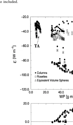
Fig. 10 shows the impact that two of the habits, columns and rosettes Mitchell et al.,
.
1996 , have on cloud and surface IR radiative properties. These habits were chosen because they have the largest differences in their optical properties. For comparison purposes, computations using the traditional equivalent volume sphere approximation are also included.
Ž . Ž
Fig. 10. Total IR cooling ´ and Fnet,lw for the three cases using various ice crystal habits labeled in the
.
Ž .
The thick, largely liquid ASC TLA reveals only a slight dependency of radiative
heatingrcooling to changes in ice habit. This is to be expected as liquid dominates the
Ž .
WP. A weak impact due to habit is also found for the thin clouds TA in the 5–15 g
y2 Ž .
m WP range. However, once ASC contain greater than 50% ice mass as in TIA , and
IWPR25 g my2, ice crystal habit begins to have a significant effect on the IR heat
y2 Ž
budget of the cloud and surface. As Fig. 10 shows,´ can be 5–20 W m smaller i.e.
.
more cloud cooling if rosette rather than columnar crystals dominate. Additionally, the
Ž .
net IR surface cooling Fnet,lw is reduced by a similar amount when rosette crystals are
assumed. This results because rosettes have a larger total extinction cross-section due to
Ž .
their branched structure Mitchell and Arnott, 1994 . Note also that equivalent volume spheres tend to have a radiative impact similar to that of rosette crystals.
In Fig. 11 differences between calculations using columns and equivalent volume spheres are shown, illustrating the influence of ice habit on the solar radiative properties
Ž .
of mixed-phase ASC. As Fig. 11a shows, clouds which are mostly ice IWPrWPR0.5
absorb 4–15 W my2
less solar radiation if columns are assumed instead of spheres. Rosette crystals also absorb more than columns; however, the difference is only between
y2 Ž .
0.5 and 1 W m not shown . This results from the high degree of sensitivity of AAto
Ž .
the relative difference in d between the crystal habits Fig. 2 .e
Clouds that consist mostly of ice show a weaker sensitivity of F than AA to
net,sw
changes in ice habit. Fig. 11b shows that Fnet,sw is 3–8 W my2 greater for columns than
for equivalent volume spheres. This result holds for a large range of m0. Similar results
are produced if spheres are replaced by rosette crystals. Overall, the total impact is not large and, therefore, ice habit may not be particularly important for computations of
Fnet,sw. Still, ice habit may be important for computing the amount of solar energy
deposited in the cloudy BL.
4.4. SensitiÕity: ice effectiÕe radius
In this section we explore the sensitivity of the cloud and surface radiative budgets to
the choice of re,i in bulk microphysical models. This is accomplished by using the IWC
from the bin microphysics and then assuming some value of r . According to Currye,i
Ž .
and Ebert 1992 , re,i;40 mm is typical for winter-time arctic low-level clouds.
Ž
However, the data from Beaufort Arctic Storms Experiment BASE, Pinto, 1998; Jiang
.
et al., 2000 , shows that mixed-phase ASC can have values up to about 300mm. Thus,
we use these two re,i values in our computations as estimates of two possible extremes
in mixed-phase ASC.
Fig. 12a–d compares ´ and Fnet,lw for TLA and TIA using both the bin and bulk
optical properties from RAMS simulations with re,is40 and 300 mm. The accurate bin
optical properties are used to illustrate the potential problems one could encounter by using a single value of to represent ice clouds in numerical models. Note that for both
Ž . Ž .
the thick liquid TLA and thick ice TIA cases, re,is300 compares best with the bin
computations. This might be expected since mixed-phase clouds produce large ice
Ž .
crystals and broad ice size spectra see Pinto, 1998; Harrington et al., 1999 , which results from the large ice supersaturations. Note the significant impact of the assumed
Ž
Ž .
Fig. 11. Contour plots of differences between column and sphere solar radiative properties. Panel a shows AA
Žcolumns –. AAŽspheres while b shows F. Ž . net,swŽcolumns – F. net,swŽspheres ..
. y2
TLA , the impact of the choice of re,i is not especially significant. For WPR40 g m ,
both ´ and F differ by as much as 5 W my2 depending on the choice of r .
net,lw e,i
Ž .
As one might expect, however, for the ice cloud TIA , the influence of re,i is much
more substantial. As Fig. 12c and d shows, both ´ and Fnet,lw and can vary by 30 to 70
Ž . Ž . Ž .
Fig. 12. Total cloud IR emission ´ and Fnet,lw for the thick liquid ASC TLA and thick ice ASC TIA
Ž . Ž . Ž . Ž .
cases. Panels a and b show the impact of various re,ifor TLA while panels c and d show the same for TIA.
mm would produce 40 W my2 too much IR cloud cooling and 70 W my2 too little
surface cooling, as compared to the calculation using the bin information. In fact, as Fig.
12d illustrates, for r of 40 mm F is positiÕe rather than negatiÕe, indicating a
e,i net,lw
warming instead of cooling for most WPs. These differences are significant even for
Ž .
thinner clouds. For the case of the thin ASC TA, not shown , in which WP ;6–14 g
my2, the choice of r produces differences of up to 20 W my2 in both ´ and F . In
e,i net,lw
fact, these large differences begin to appear for IWP as small as 8 W my2. This
illustrates the importance of correctly predicting not only IWP in numerical models, but
also re,i if one wishes to produce a consistent and accurate radiative response and energy
balance.
Fig. 13a and b shows the differences between bin computations and bulk
computa-tions with r s40mm for AAand F . Differences between the bin and bulk model
e,i net,sw
with re,is300mm are small and therefore not shown. As Fig. 13a shows, form0R0.25
and IWPrWPR0.5, solar absorption is 5 and 20 W my2 larger for re,i of 40 mm as
Ž . Ž .
Fig. 13. Contours are of differences between bin and bulk model computations. Panel a shows AA bin –AA
Žbulk, re,is40mm and panel b shows F. Ž . net,swŽbin – F. net,swŽbulk, re,is40mm ..
surface net flux is 10–30 W my2 smaller for of 40 mm. As in the case of the IR
impacts, these effects occur consistently over a broad range of IWP and are important
for IWP as small as R8 g my2.
budgets are to be computed. This is especially true for clouds composed mostly of ice, where disparities are the greatest.
5. Concluding remarks
In this paper, we have presented a parameterization for computing cloud optical properties within both bulk and bin microphysical models. While this scheme was designed specifically for RAMS, the general methodology should be adaptable to any model. The methods discussed are accurate, efficient, and correspond to the details of the microphysical scheme, including the existence of a non-spherical ice phase.
This scheme was used along with detailed, bin microphysical output from simulations
Ž .
of mixed-phase ASC Harrington et al., 1999 in order to examine the possible
importance of various microphysical assumptions in ASC on the calculation of absorp-tion, emission, and net surface fluxes in the arctic. The major results are the following.
v Compared to liquid clouds with the same WP, absorption and emission are largely
w
reduced in ice clouds due to the greater transmissivity This has also been shown by Sun
Ž .x
and Shine 1994 . In fact, the transition between predominantly liquid clouds in summer and more ice-dominated clouds in fall, winter, and spring may lead to as much as a 60
W my2 increase in IR cooling of the surface.
v Crystal habit can have a significant effect on the longwave properties of ASC,
especially when IWPR25 g my2 and the cloud is at least 50% ice. Total cloud IR
cooling and net surface fluxes can vary by as much as 20 W my2 depending on the
crystal habit.
vCrystal habit also influences the solar properties of ASC, although cloud absorption
is more sensitive than are the net surface fluxes. However, ice crystal habit influence on
Fnet is fairly small and may be neglected in many applications.
v Using ranges of ice effective radius rŽ . commonly found in the literature, our
e,i
results show that re,i has a significant impact on the radiative properties of ASC. Total
cloud longwave cooling and net surface fluxes can vary by up to 50 W my2 depending
on r . In fact, the choice of re,i e,i can determine the sign of the net surface longwaÕe flux,
leading to either a surface warming or cooling.
v The choice of r could impact the solar absorption by as much as 20 W my2 and
e,i
the surface net fluxes by up to 35 W my2.
These results have several implications for the parameterization of Arctic clouds in
Ž .
large-scale models. Most models currently predict WPs only e.g. Fowler et al., 1996
Ž
and at least three Arctic climate models tend to underpredict low-cloud WPs Curry et
.
al., 2000 . Since the radiative properties of mixed-phase clouds are sensitive to changes in cloud microstructure, information other than the LWC and IWC needs to be predicted by any GCM that includes clouds. In particular, the above results dramatically
demon-Ž
strate the fact that simply fixing a value of re,ican lead to significant errors up to 50 W
y2.
m in the radiative budget of the surface and cloudy BL. This is especially important
since studies have shown that sea ice thickness may be sensitive to a 20 W my2 or
Ž
greater change in the surface radiative budget through cloud effects Curry and Ebert,
.
1990; Curry, 1995 and that such changes may feed back into arctic cloud prediction
Acknowledgements
J. Harrington is thankful for support from the Cooperative Institute for Research in
Ž .
the Atmosphere CIRA Geosciences Project, and a joint NOAArInternational Arctic
Ž .
Research Center IARC grant. P. Olsson is grateful for support from the Alaska Experimental Forecast Facility. We would also like to thank Graeme Stephens and members of his research group at Colorado State University for useful discussions regarding the development of this parameterization.
Appendix A. Miscellaneous coefficients and functions
A.1. ADT coefficients
For reference purposes, we give the ADT and MADT coefficients in this appendix.
Ž .
The ADT extinction and absorption coefficients are given by van de Hulst, 1957 ,
Qext
Ž
D,l, m.
s2 K tD ,Ž
.
Ž
A1.
where m is the complex index of refraction and D is the diameter of a sphere.
A.2. MADT coefficients
The functions used in MADT for the modifications of the ADT absorption coefficient
Ž .
where Cir is the coefficient that corrects for internal reflectionrrefraction, Cres is the
Ž .
coefficient that corrects for resonance tunneling, and the other variables in Eq. A4 are given by,
The MADT modifications to the extinction coefficient include resonance tunneling
Žgiven above and a term that accounts for edge effects Mitchell, 2000 ,. Ž .
y2r3
Qedges2
Ž
pk.
1yexpŽ
y0.06pk.
.Ž
A5.
The edge effect term, Qedge, corrects for the fact that grazing radiation reflected from the
edge of a drop may interfere with grazing radiation that was not reflected.
A.3. MADT integral solutions
Ž .
By examining the integral over size in Eq. 2 ,
`
bext ,abss
H
A D QŽ .
ext ,absŽ
D, m,l. Ž .
n D d D,Ž
A6.
0
along with the MADT and ADT functions given above it is evident that the integrals over size have the following general form,
`p
2 b yc D
ks
H
D K xD aD eŽ
.
n D d D,Ž .
Ž
A7.
4
0
where the general variables x, a, b, and c are independent of size and the K function is
Ž .
defined by Eq. A3 . The solution to the integral k can be shown to be,
k
Ž
D , x , a, b, c,n n.
sA k1q2 ReŽ
k2qk3.
,Ž
A8.
where A is the total cross-sectional area. Note the similarity between the k-function and
Ž .
the K-function for ADT given by Eq. A3 .
The use of this solution allows one to write the total extinction and absorption
Ž . Ž . Ž Ž ..
compactly as in Eqs. 6 and 7 . The Q functions for the absorption Eq. 7 are given
by the following,
Qabss1yk
Ž
D , 0, 1, 0, y,n n.
,Qirsk
Ž
D , 0, a , 0, y,n ir n.
ykŽ
D , 0, a , 0, 2 y,n ir n.
,X X
Qressk
Ž
D , 0, fn res, m,ek ,n.
ykŽ
D , 0, fn res, m, yqek ,n.
,Ž
A9.
where we have defined the following coefficients,
8pni ra X 1
ys , fress m m ym, ks .
Ž Ž ..
For the extinction coefficient Eq. 6 , the Q functions become,
Qexts2k
Ž
D , t , 1, 0, 0,n n.
,For the absorption, one needs to solve the general integral given by Eq. 9 . Using the
Ž .
empirical form for the projected area given in Mitchell and Arnott 1994 ,
P L
Ž .
sB LapqC Lbp,Ž
A11.
p p
Ž .
and using Qabs,i with the linear parameterization of de saqbL , one can analytically
Ž .
solve the integral over size as shown in Mitchell and Arnott 1994 . Using this
Ž .
information allows one to write the absorption compactly as given by Eq. 10 . The average functions in this equation are given by,
Nt a
The various functions defined above are given by the following relations,
cl ,h
Ž
L , a, b, c, x ,n n.
References
Auer, A.H., Veal, D.L., 1970. The dimension of ice crystals in natural clouds. J. Atmos. Sci. 27, 919–926. Boers, R., Mitchell, R.M., 1994. Absorption feedback in stratocumulus clouds: Influence on cloud top albedo.
Tellus 46A, 229–241.
Curry, J.A., 1986. Interactions among turbulence, radiation and microphysics in Arctic stratus clouds. J. Atmos. Sci. 43, 90–106.
Curry, J.A., 1995. Interactions among aerosols, clouds, and climate of the Arctic Ocean. Total Environ. 160–161, 777–791.
Curry, J.A., Herman, G.F., 1985. Infrared radiative properties of summertime arctic stratus clouds. J. Clim. Appl. Meteor. 24, 525–538.
Curry, J.A., Ebert, E.E., 1990. Sensitivity of the thickness of arctic sea ice to the optical properties of clouds. Ann. Glaciol. 14, 43–46.
Curry, J.A., Ebert, E.E., 1992. Annual cycle of radiation fluxes over the Arctic Ocean: sensitivity to cloud optical properties. J. Clim. 5, 1267–1280.
Curry, J.A., Rossow, W.B., Randall, D., Schramm, J.L., 1996. Overview of Arctic cloud and radiation characteristics. J. Clim. 9, 1731–1764.
Curry, J.A., Pinto, J.O., Benner, T., Tschudi, M., 1997. Evolution of the cloudy boundary layer during the autumnal freezing of the Beaufort sea. J. Geophys. Res. 102, 13851–13860.
Curry, J.A., Hobbs, P.V., King, M.D., Randall, D.A., Minnis, P., Isaac, G.A., Pinto, J.O., Uttal, T., Bucholtz, A., Cripe, D.G., Gerber, H., Fairall, C.W., Garrett, T.J., Hudson, J., Intrieri, J.M., Jakob, C., Jensen, T., Lawson, P., Marcotte, D., Nguyen, L., Pilewskie, P., Rangno, A., Rogers, D.C., Strawbridge, K.B., Valero, F.P.J., Williams, A.G., Wylie, D., 2000. FIRE arctic cloud experiment. Bull. Am. Meteorol. Soc. 81, 5–29. Doutriaux-Boucher, M., Buriez, J.C., Brogniez, G., Labonnote, L.C., 2000. Sensitivity of retrieved POLDER
directional cloud optical thickness to various ice particle models. Geophys. Res. Lett. 27, 109–112. Duda, D.P., Stephens, G.L., Stevens, B., Cotton, W.R., 1996. Effects of aerosol and horizontal inhomogeneity
on the broadband albedo of marine stratus: numerical simulations. J. Atmos. Sci. 53, 3757–3769. Ebert, E.E., Curry, J.A., 1992. A parameterization of ice cloud optical properties for climate models. J.
Geophys. Res. 97, 3831–3836.
Edwards, J.M., Slingo, A., 1996. Studies with a flexible new radiation code: Part I. Choosing a configuration for a large scale model. Q. J. R. Meteorol. Soc. 122, 689–719.
Feingold, G., Stevens, B., Cotton, W.R., Walko, R.L., 1994. An explicit cloud microphysicsrLES model designed to simulate the Twomey effect. Atmos. Res. 33, 207–234.
Ferrier, B.S., 1994. A double-moment multi-phase four-class bulk ice scheme: Part I. Description. J. Atmos. Sci. 51, 249–280.
Fowler, L.D., Randall, D.A., Rutledge, S.A., 1996. Liquid and ice microphysics in the CSU general circulation model: Part I. Model description and simulated microphysical processes. J. Clim. 9, 489–529.
Fu, Q., Liou, K.N., 1992. Parameterization of the radiative properties of cirrus clouds. J. Atmos. Sci. 50, 2008–2025.
Grenfell, T.C., Warren, S.G., 1999. Representation of a nonspherical ice particle by a collection of independent spheres for scattering and absorption of radiation. J. Geophys. Res. 104, 31697–31709. Harrington, J.Y., 1997. The Effects of Radiative and Microphysical Processes on Simulated Warm and
Transition Season Arctic Stratus. PhD thesis, Colorado State University, Ft. Collins CO, 80523, USA. Harrington, J.Y., Olsson, P.Q., 1999. Influence of cloud microphysical processes on the dynamical evolution
of the boundary layer during off-ice flow. Third Conference on Coastal Atmospheric and Oceanic Prediction and Processes. New Orleans, LA, 3–5 Nov. American Meteorological Society.
Harrington, J.Y., Reisin, T., Cotton, W.R., Kreidenweis, S.M., 1999. Cloud resolving simulations of Arctic stratus: Part II. Transition-season clouds. Atmos. Res. 51, 45–75.
Harrington, J.Y., Feingold, G., Cotton, W.R., 2000. Radiative impacts on the growth of a population of drops within simulated summertime arctic stratus. J. Atmos. Sci. 57, 766–785.
Herman, G., Goody, R., 1976. Formation and persistence of summertime Arctic stratus clouds. J. Atmos. Sci. 33, 1537–1554.
Hu, Y.X., Stamnes, K., 1993. An accurate parameterization of the radiative properties of water clouds suitable for use in climate models. J. Clim. 43, 784–801.
Intrieri, J., Eberhard, W.L., Alverez II, R.J., Sandberg, S.P., McCarty, B.J., 1999. Cloud statistics from LIDAR at SHEBA. Fifth Conference on Polar Meteorology and Oceanography, Dallas, TX, 10–15 Jan. American Meterological Society.
Jiang, H., Cotton, W.R., Pinto, J.O., Curry, J.A., Weissbluth, M.J., 2000. Sensitivity of mixed-phase arctic stratocumulus to ice forming nuclei and large-scale heat and moisture advection. J. Atmos. Sci. 57, 2105–2117.
Kogan, Y.L., Khairoutdinov, M.P., Lilly, D.K., Kogan, Z.N., Liu, Q., 1995. Modeling of stratocumulus cloud layers in a large eddy simulation model with explicit microphysics. J. Atmos. Sci. 52, 2293–2940. Labonnote, L.C., Brogniez, G., D.-Boucher, M., Buriez, J.-C., 2000. Modeling of light scattering in cirrus
clouds with inhomogeneous hexagonal monocrystals. Comparison with in-situ and ADEOS-POLDER measurements. Geophys. Res. Lett. 27, 113–116.
Lynch, A.H., Chapman, W.L., Walsh, J.E., Weller, G., 1995. Development of a regional climate model of the western Arctic. J. Clim. 8, 1555–1570.
Meyers, M.P., Walko, R.L., Harrington, J.Y., Cotton, W.R., 1997. New RAMS cloud microphysics parameter-ization: Part II. The two-moment scheme. Atmos. Res. 45, 3–39.
Mitchell, D.L., 1994. A model predicting the evolution of ice particle size spectra and radiative properties of cirrus clouds: Part I. Microphysics. J. Atmos. Sci. 51, 797–816.
Mitchell, D.L., 2000. Parameterization of the Mie extinction and absorption coefficients for water clouds. J. Atmos. Sci. 57, 1311–1326.
Mitchell, D.L., Arnott, W.P., 1994. A model predicting the evolution of ice particle size spectra and radiative properties of cirrus clouds. Part II: Dependence of absorption and extinction on ice crystal morphology. J. Atmos. Sci. 51, 817–832.
Mitchell, D.L., Zhang, R., Pitter, R.L., 1990. Mass-dimensional relationships for ice particles and the influence of riming on snowfall rates. J. Appl. Meteorol. 29, 153–163.
Mitchell, D.L., Macke, A., Liu, Y., 1996. Modeling cirrus clouds. Part II: Treatment of radiative properties. J. Atmos. Sci. 53, 2967–2988.
Olsson, P.Q., Harrington, J.Y., 2000. Dynamics and energetics of the cloudy boundary layer in simulations of off-ice flow in the marginal ice zone. J. Geophys. Res. 105, 11889–11899.
Olsson, P.Q., Harrington, J.Y., Feingold, G., Cotton, W.R., Kreidenweis, S.M., 1998. Exploratory cloud-re-solving simulations of boundary layerA rctic stratus clouds: Part I. Warm Season clouds. Atmos. Res. 47, 573–597.
Pinto, J.O., 1998. Autumnal mixed-phase cloudy boundary layers in the Arctic. J. Atmos. Sci. 55, 2016–2038. Reisin, T., Levin, Z., Tzivion, S., 1996. Rain production in convective clouds as simulated in an axisymmetric
model with detailed microphysics: Part I. Description of the model. J. Atmos. Sci. 53, 497–519. Ritter, B., Geleyn, J.-F., 1992. A comprehensive radiation scheme for numerical weather prediction models
with potential applications in climate simulations. Mon. Wea. Rev. 120, 303–325.
Royer, J.F., Planton, S., Deque, M., 1990. A sensitivity experiment for the removal of Arctic sea ice with the French spectral general circulation model. Clim. Dyn. 5, 1–17.
Rutledge, S.A., Hobbs, P.V., 1984. The mesoscale and microscale structure and organization of clouds and precipitation in midlatitude cyclones: VIII. A model for the ‘‘seeder–feeder’’ process in warm-frontal rainbands. J. Atmos. Sci. 40, 1185–1206.
Slingo, A., Schrecker, H.M., 1982. On the shortwave properties of stratiform water clouds. Q. J. R. Meteorol. Soc. 108, 407–426.
Stackhouse, P.W., Stephens, G.L., 1991. A theoretical and observational study of the radiative properties of cirrus: results from FIRE 1986. J. Atmos. Sci. 48, 2044–2059.
Stephens, G.L., 1978. Radiation profiles in extended water clouds: II. Parameterization schemes. J. Atmos. Sci. 35, 2123–2132.
Stevens, B., Feingold, G., Cotton, W.R., Walko, R.L., 1996. Elements of the microphysical structure of numerically simulated nonprecipitating stratocumulus. J. Atmos. Sci. 53, 980–1007.
Sun, Z., Shine, K.P., 1995. Parameterization of ice cloud radiative properties and its application to potential climatic importance of mixed-phase clouds. J. Clim. 8, 1874–1888.
Takano, Y., Liou, L.-N., 1989. Solar radiative transfer in cirrus clouds: Part I. Single-scattering and optical properties of hexagonal ice crystals. J. Atmos. Sci. 46, 3–19.
Tzivion, S., Feingold, G., Levin, Z., 1989. The evolution of rain-drop spectra. Part II: Collisional collectionrbreakup and evaporation in a rain shaft. J. Atmos. Sci. 46, 3312–3327.
Utall, T., Orr, B., Hazen, D., Otten, J., Ryan, M., Shupe, M., Martner, B., 1999. Cloud boundary statistics for SHEBA from mm-wave cloud radar. Fifth Conference on Polar Meteorology and Oceanography, Dallas, TX, 10–15 Jan. American Meteorological Society.
van de Hulst, H.C., 1957. Light Scattering by Small Particles. Dover, New York.
Walko, R.L., Cotton, W.R., Meyers, M.P., Harrington, J.Y., 1995. New RAMS cloud microphysics parameter-ization: Part I. The single moment scheme. Atmos. Res. 38, 29–62.
Wielicki, B.A., Suttles, J.T., Heymsfield, A.J., Welch, R.M., Spinhirne, J.D., Wu, M.-L.C., Starr, D., Parker, L., Arduini, R.F., 1990. The 27–28 October 1986 FIRE IFO cirrus case study: comparison of radiative transfer theory with observations by satellite and aircraft. Mon. Wea. Rev. 118, 2356–2376.