MACHINE LEARNING BASED ROAD DETECTION FROM HIGH RESOLUTION
IMAGERY
aYe Lv ,bGuofeng Wang,cXiangyun Hu
a
School of Remote Sensing and Information Engineering, Wuhan University, P.R. China - [email protected] bChina Highway Engineering Consulting Corporation, Beijing, P.R.China - [email protected]
c
School of Remote Sensing and Information Engineering, Wuhan University, P.R. China - [email protected]
ICWG III/VII
KEY WORDS: Road Extraction, Machine Learning, Image Segmentation, ROIs, Geometric Statistics Analysis, Road Feature
ABSTRACT:
At present, remote sensing technology is the best weapon to get information from the earth surface, and it is very useful in geo-information updating and related applications. Extracting road from remote sensing images is one of the biggest demand of rapid city development, therefore, it becomes a hot issue. Roads in high-resolution images are more complex, patterns of roads vary a lot, which becomes obstacles for road extraction. In this paper, a machine learning based strategy is presented. The strategy overall uses the geometry features, radiation features, topology features and texture features. In high resolution remote sensing images, the images cover a great scale of landscape, thus, the speed of extracting roads is slow. So, roads’ ROIs are firstly detected by using Houghline detection and buffering method to narrow down the detecting area. As roads in high resolution images are normally in ribbon shape, mean-shift and watershed segmentation methods are used to extract road segments. Then, Real Adaboost supervised machine learning algorithm is used to pick out segments that contain roads’ pattern. At last, geometric shape analysis and morphology methods are used to prune and restore the whole roads’ area and to detect the centerline of roads.
1. INTRODUCTION
As the increasing development of information industry and tech-nology, the relationship between humans and geoinformation is tighter. Extracting geoinformation accurately and effectively has now been the shared goal of all information science researcher-s. Nowadays, photogrammetry, remote sensing and computer vi-sion technologies can provide us with powerful tools to collect ,process and analyze massive amount of geo-spatial information, thus, giving a strong support for city development.
Extracting objects from remote sensing images has always been the main goal of computer vision. And because road has been the main subject in traffic analysis, city planning, disaster response and many other important issues, road extraction plays an impor-tant role in the research of city development. At present, high geometry resolution, high spectral resolution, and high radiation resolution remote sensing images give us more detailed informa-tion of our living environment, providing us with better quality research data, but in the mean time, it brings greater challenge as a result of greater computation complexity.
In recent twenty years, various kinds of road extraction meth-ods have been proposed. Many research laboratories have done contributions to road extraction. Such as McKeown laborato-ry in America, ”Amobe” Program in Switzerland,Karl-Franzens-Universitt Graz in Germany, Wuhan University, The PLA Infor-mation Engineering University and ATR laboratory of National University of Defense Technology in China and so on.
Roads’ patterns are complex in high resolution images. Nor-mally, roads’ geometry feature, radiation feature, topology fea-ture ,contextual feafea-ture are used for road extraction (Vosselman and Knecht, 1995). Indeed, there is a great number of roads detection methods, such as, mathematical morphology method-s (Singh and Garg, 2013), template matching methodmethod-s (Cheng et al., 2011), snake model methods (Yang and Zu, 2009), dynamic
programming methods (Sujatha and Selvathi, 2015), segmenta-tion methods (Song and Civco, 2004), edge detecsegmenta-tion (Sirmacek and Unsalan, 2010) , perceptual organization methods (Gamba et al., 2006), machine learning methods (Wang et al., 2006), line detection methods, line tracking methods (Bicego et al., 2003) and so on. To improve the robustness of roads detection, vari-ous auxiliary data of different types is being used, for example, by using combination of Lidar cloud points and remote sensing images (Chen et al., 2009), or combination of DEM and remote sensing images (Hinz et al., 2001).
In this paper, the main detection strategy is shown as follows. Firstly, roads’ ROIs are detected using canny edge detection and hough line detection method. Secondly, do image segmentation by mean-shift algorithm integrated with iterative marker-based watershed area merging algorithm. Thirdly, train a classifier by Adaboost algorithm using SIFT texture and color information, then use the classifier to select segments containing road patterns. Finally, by shape analysis and morphology methods, roads areas and center lines are extracted. Overall, image segmentation, fea-ture extraction, machine learning, shape analysis and morphology methods are adopted for road detection in this paper. The main frame is shown in Figure 1.
2. REGION OF INTEREST EXTRACTION 2.1 Introduction
ROIs extraction contributes a lot to roads segmentation selection, this process helps to narrow down the searching space and cut down the time for feature calculation and analysis. In this part, Canny operator combined with Hough line detection algorithm is used.
High-resolution Remote Sensing Image
Meanshift Segmentation
Iterative Marker-based Watershed Small Area
Removal
Retrieve Segments in Road ROIs
Retrieve Segments Containing Roads’ Pattern Canny Edge Detection
Hough Line Detection
Road ROIs Extraction
Sampling Training Data
Acquire Sift Feature Points of both
Positive and Negative Samples
Training by Adaboosting
Algorithm
Shape Analysis Constraints
Morphological Pruning
Roads’ texture and radiation constraints
Detecting Centerlines by Morphology Thinning
Figure 1. Road Extraction MainFrame
road edges, road lanes and isolation belts. In the meantime, these high gradient area has a length. By detecting these features, ROIs can extracted.
There are many edge detection operators, such as Roberts oper-ator, Prewitt operoper-ator, Sobel operoper-ator, Kirsch operoper-ator, Nevitia operator, laplace operator, Canny operator, Marr-Hildreth opera-tor and so on. Among them, Canny is regarded as the most robust operator.
Canny operator is brought out as a multi-level edge detector by John F.Canny in 1986 (J, 1986). This operator can depress noise in some degree, and effectively detect edges. So, it is of remark-able effect to detect roads edge features.
Hough transformation is an effective vote based parameter esti-mator. According to the points correspondence in image space and parameter space, Hough transformation changes the ques-tion of feature detecques-tion into accumulaques-tion statistics in parame-ter space. Hough transform can be adopted to detect arbitrary shapes (Ballard, 1987) such as, lines, circles, ellipses, parabol-ic curves and so on. By detecting lines, the strong indparabol-icators of roads existence.
2.2 Experiment and Analysis
Select 24 depth2000×900BMP image as research data. As shown in 2(a), the image contains many ground feature elements such as buildings, fields, roads, trees, grass, bare land and so on. The main roads width is about 28 pixels. In the image, roads edges, road lanes and cars can be seen.
To begin with, 3×3 Gaussian filter is applied to smooth the image. Then, the image of 3 channels is transformed into image
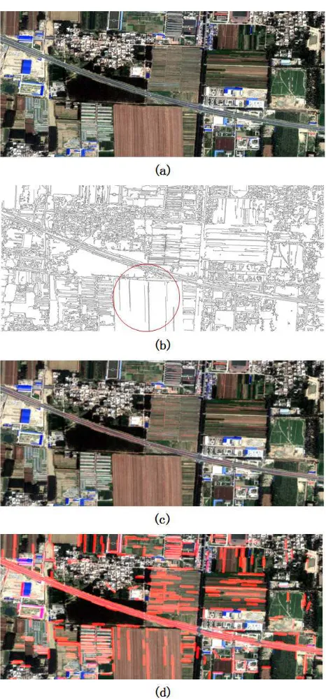
Figure 2. (a)Original image(b)Canny edge detection(c)Hough line segments detection(d)Hough line buffer
with 1 channel according to human visual property, the equation is shown in 1 below.
GreyV alue= 0.299R+ 0.587G+ 0.114B (1)
Then, adopt Canny operator, setting high threshold and low thresh-old parameter to be 125 and 40 separately. The edges are shown in Figure 2(b).
hough lines are presented, step of length is 1 pixel, step of line direction is 0.5 degree. Result of Hough line detection result is shown in Figure 2(c).
It shows that major roads parts and lanes are detected. Besides, other line pattern in the fields and straight edges of buildings are detected. Based on these line segments, ROI buffers containing straight roads can be extracted, shown in Figure 2(d). The buffers cover most of the roads.
3. IMAGE SEGMENTATION AND MERGING 3.1 Introduction
Image segmentation partition the image into blobs of similar prop-erties. It is an important process between image processing and image analysis. Image segmentation methods can be categorized into the following groups: 1. Thresholding based method, such as image binarization, OSTU thresholding method. 2. Region based method, such as region growth method, splitting and merg-ing method. 3. Edge based method, such as LoG operators, Can-ny operators. 4. Other specific theory based method, such as cluster analysis, fuzzy set theory, genetic coding method and so on. In this paper, Mean Shift segmentation algorithm is used for segmentation and Iterative Marker-based Watershed algorithm is used for small segments removal.
3.2 MeanShift Image Segmentation
Meanshift algorithm is based on non-parametric kernel densi-ty estimation, it is brought out first by Fukunaga (Fukunaga K, 1975) in 1975. Fukunaga named shift vector pointing to the max-imum probility density to be meanshift vector. Comaniciu (D Co-maniciu, 1999) proved the convergency of meanshift algorithm, and applied it to image smoothing, image segmentation (Comani-ciu and Meer, 1997) and moving object tracking.
For color image, radius of grey values of three channels are cor-respond to color field parameter r, radius of pixel indexes of row and column are correspond to spatial field parameter s. hs and hr are the bandwidth of s and r separately. The main steps are as fol-lows. 1) Assignyi,j=xi, i is the index of pixels, j is the iteration
times, beginning from j=1; 2) calculatingyi,j+1=yi,j+mh(x)
un-tilyi,jconverged toyi,c, log valueyi,c. On abovemh(x)is the
meanshift vector; 3) Assignzi =yi,c; 4) In the range of hs and
hr, assign all the pixels that converged tozito be{Cp}p=1...m,
that is, assign all the pixels converged tozito be the same class.
5) Mark the class, and erase the segments that have too few pix-els;
3.3 Iterative Marker-Based WaterShed small Blobs Removal In the last 70s century, C. Digabel and H.Lantuejoul applied wa-tershed algorithm in digital image processing. Due to the limita-tion of tremendous computalimita-tion complexity, watershed algorithm was not widely used, but regarded as a binarization method. Af-ter the further research by Luc Vincent (Vincent and Soille, 1991) and S.Beucher (Beucher, 1994), computational complexity of wa-tershed algorithm is optimized a lot and thus, wawa-tershed started to be widely used.
In 1992, Meyer introduced a non-parametric Marker-based Wa-tershed algorithm (Meyer, 1992). The basic idea is to take gra-dient image as a landforms in geology. Each pixels value in the image represents the height above sea level. At each locally min-imum height, prick a pole. Then, sink the model in the water. As
the water is deeper and deeper, water begins to spread out from the poles forming local pools.
To eliminate over segmentation caused by small variation in gray value, gradient function can be modified as in equation 2.
g(x, y) =max(grad(f(x, y)), g) (2)
g stands for threshold, grad stands for calculating gradient oper-ation. To eliminate noise and irregularity influence, an iterative non-parameter Marker-based Watershed algorithm is adopted to eliminate small blobs. Normally, it only takes two or three times iteration to achieve a good result. Iterative marker-based water-shed algorithm is shown as follows. Firstly, set the threshold T for pixel number, such as 20. Then, set iteration times to be N, such as 2 or 3. Thus, the threshold ti for each iteration time i can be defined, that is, ti=T/(N-i+1), the input of iteration i+1 is the output of iteration i. As for pixels at the boundary of differen-t segmendifferen-ts. They can be assigned differen-to differen-the nearby segmendifferen-t whose average pixel value is closest to them. The advantage of applying watershed merging strategy is that: 1) Merging starts from the pixel with minimum value contrast against it, it avoids looking for pixels that have closest value. 2) No need to look for adjacent segments and no need to manage the adjacency list. 3) Effec-tive when dealing with lanes or cars on road. The disadvantage of this method is that objects with very small width will be lost. However, the roads width is large enough not to be erased.
3.4 Experiment and Analysis
Apply the meanshift filter on the color image, setting the hs to be 8 and hr to be 10. In each segment, assign the average color of pixels in it to each pixel within. After applying the filter, the image will be a little blurred shown in Figure 3(a).
D
E
Figure 3. (a)Local meanshift filter result (b)Local origin image
Overall result is shown in Figure 4(a).
Merge the small color contrast segments according to equation 3. Src(x,y) is the image. x,y is the coordinates of the point to be modified,x′y′are the 4 neighborhood of pixel (x,y). loDiff and
upDiff are two threshold. In the experiment, set both loDiff and upDiff to be 5.
src(x′, y′)−loDif f≤src(x, y)≤src(x′, y′) +upDif f
(3)
D
E
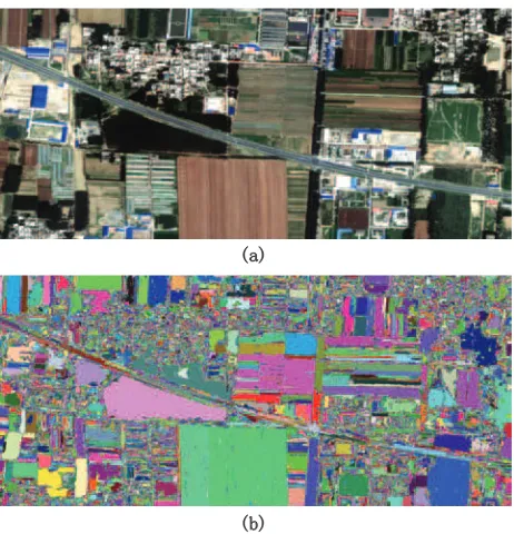
Figure 4. (a)Meanshift filter result (b)Meanshift image segmen-tation
is a gradual change in the radiation along the road, so, the road is partitioned into different parts.
Using method based on Iterative Marker-based Watershed, smal-l segments can be effectivesmal-ly esmal-liminated, incsmal-luding unnecessary details such as cars. Setting threshold T to be 80 and iteration times N to be 2. Some too narrow objects will be eliminated shown in Figure 5(a) and Figure 5(b).
Figure 5(c)(d) shows two times small segments removal effects. The color of the segment is the average color of the pixels within. The figure shows, segments whose pixel number is above 40 less than 80 will not be merged to other segments.
D E
F G
Figure 5. (a)Origin Image (b)First merging result (c)First merg-ing result (d)Second mergmerg-ing result
Overall segmentation results are shown in Figure 6
After segmentation, extract the segments who has 60% area insid-e thinsid-e ROI buffinsid-ers. Thinsid-e rinsid-esult is shown in Figurinsid-e 7, sinsid-egminsid-ents with line patterns are reserved as well as some other small segments which will be eliminated afterward.
D
E
Figure 6. (a)First watershed iteration result (b)Second watershed iteration result
Figure 7. Segments in ROIs
4. ROAD SEGMENTS EXTRACTION 4.1 Introduction
Roads have unique texture patterns involving cars, lanes and pas-sengers. To retrieve segments with road patterns, method that combines SIFT and AdaBoost algorithm is used. SIFT algorithm creatively computes key points according to DOG and constructs 128 dimensions local invariant feature descriptor to analyze the local feature pattern. With SIFT feature descriptor and 3 color channels, patterns of roads are sent to AdaBoost algorithm. Af-ter training the classifier, the classifier can be used to select road segments.
4.2 Texture Analysis
Texture analysis is one of the hottest issue, and is applied in many fields. Such as object detection, remote sensing image analysis, products checking and medical image analysis. Common extrac-tion methods includes: construcextrac-tion method, statistics method, frequency spectrum method and model method.
1994). Besides, it is adaptive to light variation and image distor-tion, and has high differentiating capability. SIFT has mainly two parts, they are key points detection and feature description.
As for key points detection. First, subsample the image using different scale Gaussian kernel function to get Gaussian image pyramid. Second, compute DOG by adjacent level images. Third, compare the points with neighbor points in current and adjacent level images, and set local extremes to be the key points and log their positions and scales. For better precision, curved surface fitting can be used.
As for descriptor representation, take the key point of its scale as center, then take16×16neighbor pixels and divide these 256 pix-els into4×4sub-blocks. Calculate gradient direction histogram (8 main direction from 0 to 360 degree) for each sub-block. Then, rearrange the order forming4×4×8 = 128dimensions vector.
4.3 Adaboost Training
In the field of machine learning, after Valiant published paper (Valiant, 1984). Many researchers turned focus on the PAC (Prob-ably Approximately Correct) learning model.
Kearns and Valiant (Kearns et al., 1994) said that, in PAC learning model, if there exists a polynomial learning algorithm for concept recognition with high correct rate, then these concepts are strong-ly learnable. On the contrary, if the correct rate is onstrong-ly a little bet-ter than random guess, then these concepts are weakly learnable. Kearns and Valiant proved the equality of weakly learnable algo-rithm and strongly learnable algoalgo-rithm, that is, weakly learnable model can be strengthened into strongly learnable algorithm.
In 1995, Freund and Schapire brought out Adaboost algorith-m. AdaBoost algorithm is a supervised learning algorithm, it cascades many weak classifiers into a very effective classifier. Though these weak classifiers may be simple, but only if their result is a little better than random guess, they can be cascaded into strong classifier with Boosting methods. Boosting algorithm has many variants, including Discrete AdaBoost, Real AdaBoost, LogitBoost and Gentle AdaBoost. To reduce the computation time, samples already being classified with very high confidence can be excluded from training set (Freund, 1995).
4.4 Experiment and Analysis
There are mainly four steps for classification. 1) Sample points selection.2) Feature descriptor construction.3) Classifier Train-ing.4) Classification of the key points in ROIs.
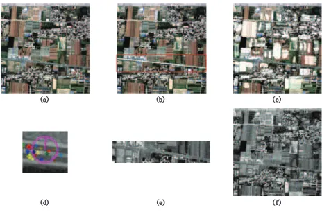
1)Manually select positive and negative samples range from which samples are extracted. To improve the classifier, the sample types should be rich enough. A2000×2000image is used. In the range, SIFT key points extraction algorithm is applied to extract key points. The Figure 8(a)(b)(c) below shows the original sam-pling image, positive and negative samsam-pling range.
2)Calculate the feature descriptor of the extracted key points in both positive and negative range. Then, add the value of three color channels to the end of the descriptor (Figure 9). Use this descriptor to extract positive and negative samples from positive range and negative range. Figure 9(d) shows SIFT key points, ra-dius of the circle represents the scale and the rara-dius direction rep-resents the direction. The experiment is done by using OpenCV. SIFT parameters are set as follows. The number of layers in each octave is 3, the contrast threshold used to filter out weak features is 0.01, the threshold used to filter out edge-like features is 20.
D E F
G H I
Figure 8. (a)Original image used for training classifier (b)Positive sampling range (c)Negative sampling range (d)Key point repre-sentation (e)Positive SIFT key point samples (f)Negative SIFT key point sample
1 2 3 128 1 2 3
128 SIFT Descriptor 3 Color channels
Figure 9. Descriptor
Sigma of Gaussian filter is 1.2. The second and the third parame-ter should not be too high in order to get enough training samples. Figure 9(e)(f) show the positive and negative sample key points separately. There are 1198 positive samples and 37748 negative samples.
3)Real AdaBoost is adopted, set the weak classifier to be 200, when any samples correct rate is above 0.999, it is removed from the training set. After the classifier is retrieved, it can be applied to our original image. First, key points in road ROIs are detected, then the key points with road texture can be extracted using clas-sifier. The result is shown in Figure 10. The green points are the key points classified as points with road texture pattern. Precision rate is very high, only 9 points are wrongly classified as non-road pattern points.
Figure 10. Prediction
Figure 11.
Figure 11. Result of road segments extraction
5. SHAPE ANALYSIS AND MORPHOLOGY OPERATION
5.1 Introduction
Road has a special shape, it is a long stripe with width. By using shape analysis, the non-road segments can be erased. In this pa-per, three norms are used. After shape analysis, morphology can be used to prune road segments and extract roads
5.2 Shape Analysis 1)Area S
In high resolution image, roads are connected and with a large area. Small non-road object such as buildings can be erased. The threshold is determined by image resolution.
2)Length width ratio R In high resolution image, roads are stripe objects, so the length width ratio of its minimum area bounding rectangle(MABR)(Figure 12) is large.
R=LM ABR/WM ABR (4)
In 4,LM AERandWM AERare the length and the width of roads
minimum area bounding rectangle.
F =S/SM ABR (5)
S is the area of road,SM ABRis the area of minimum area
bound-ing rectangle, soF ≤1.0. Fullness rate is used to extract com-plex road network, where R of roads MABR is not large but F is very small. If it satisfies the equation 6, the area is determined as road.TS,TF,TRare thresholds for S, F and R.
Mathematical morphology operation is a theory analyzing spatial structure. It is based on set theory, integral theory and grid alge-bra. The biggest feature of it is to use shifting and logical opera-tion which is fast and agile rather than other complex operaopera-tion. In this paper, the open operation is used to prune the coarse edge, then, close operation is used to seal the holes in roads. Finally, thinning operation is used to extract the center line of road.
Figure 12. MABR example
5.4 Experiment and Analysis
In the part of shape analysis,TS = 1000,TF = 0.2,TR = 7. In
the Figure 13(b), the MABR of the main road is shown in yellow color. Its R reaches 17.9, its fullness reaches 0.21 and the area of road reaches 52023 pixels. Other small erased components parameters are listed below in the order(R,S,F).
(5,939,0.46),(3.75,1456,0.72),(9.89,644,0.92),(3.4,779,0.65).
In the part of morphology, circle operation element is used. Ra-dius for open operation is 5 which is small in order not to split the road, and radius for close operation is 15 which is bigger in or-der to fuse some roads that are broken.Figure 13(c)(d) shows the pruned road area and the extracted center line of road. Figure 14 shows the final result overlapped on the original image.
5.5 Result and Conclusion
In this paper, we present a work flow of possible road extraction strategy. However, there is still great potential to upgrade each part. ROIs extraction is a good preliminary for further operations. Image segmentations, machine learning techniques together with shape constraints can be effective to choose possible road areas. The morphology operation can be used for segments tuning and centerline detection pretty easily. Overall, this strategy is useful for road extraction applications.
REFERENCES
Ballard, D. H., 1987. Generalizing the hough transform to detect arbitrary shapes.Pattern Recognition13(81), pp. 111–122.
Beucher, S., 1994. Watershed, hierarchical segmentation and wa-terfall algorithm.Computational Imaging & Vision2, pp. 69–76.
Bicego, M., Dalfini, S., Vernazza, G. and Murino, V., 2003. Auto-matic road extraction from aerial images by probabilistic contour tracking. In:Proceedings / ICIP ... International Conference on Image Processing, pp. III–585–8 vol.2.
Chen, Y., Su, W., Li, J. and Sun, Z., 2009. Hierarchical object oriented classification using very high resolution imagery and l-idar data over urban areas. Advances in Space Research43(7), pp. 1101–1110.
Figure 13. (a)Before shape analysis (b)After shape analysis (c)Pruned road (d)Extracted center line of road
Comaniciu, D. and Meer, P., 1997. Robust analysis of feature s-paces: color image segmentation. In:Proceedings / CVPR, IEEE Computer Society Conference on Computer Vision and Pattern Recognition. IEEE Computer Society Conference on Computer Vision and Pattern Recognition, pp. 750–755.
D Comaniciu, P. M., 1999. Mean shift analysis and applications. IEEE International Conference on Computer Vision.
Freund, Y., 1995. Boosting a weak learning algorithm by
majori-Figure 14. Extracted center line on origin image
ty.IEEE Trans on Acoustics Speech & Signal Processing121(2), pp. 256–285.
Fukunaga K, H. L., 1975. The estimation of the gradient of a density function, with applications in pattern recognition. Infor-mation Theory IEEE Transactions on21(1), pp. 32–40.
Gamba, P., Dell’Acqua, F. and Lisini, G., 2006. Improving urban road extraction in high-resolution images exploiting directional filtering, perceptual grouping, and simple topological concepts. Geoscience & Remote Sensing Letters IEEE3(3), pp. 387–391.
Hinz, S., Baumgartner, A., Steger, C., Mayer, H., Eckstein, W., Ebner, H. and Radig, B., 2001. Road extraction in rural and urban areas.Ias.informatik.tu.
J, C., 1986. A computational approach to edge detection.Pattern Analysis & Machine Intelligence IEEE Transactions on pami-8(6), pp. 679–698.
Kearns, M., Li, M. and Valiant, L., 1994. Learning boolean for-mulas. Journal of the Acm41(6), pp. 1298–1328.
Lindeberg, T., 1994. Scale-space theory in computer vision. Springer Berlin256, pp. 349–382.
Lowe, D. G., 2004. Distinctive image features from scale-invariant keypoints. International Journal of Computer Vision 60(2), pp. 91–110.
Meyer, F., 1992. Color image segmentation. In: Image Pro-cessing and its Applications, 1992., International Conference on, pp. 303–306.
Singh, P. P. and Garg, R. D., 2013. Automatic road extraction from high resolution satellite image using adaptive global thresh-olding and morphological operations.Journal of the Indian Soci-ety of Remote Sensing41(3), pp. 631–640.
Sirmacek, B. and Unsalan, C., 2010. Road network extraction using edge detection and spatial voting. In:Pattern Recognition (ICPR), 2010 20th International Conference on, pp. 3113–3116.
Song, M. and Civco, D., 2004. Road extraction using svm and image segmentation. Photogrammetric Engineering & Remote Sensing70(12), pp. pgs. 1365–1372.
Sujatha, C. and Selvathi, D., 2015. Connected component-based technique for automatic extraction of road centerline in high res-olution satellite images.Eurasip Journal on Image & Video Pro-cessing2015(1), pp. 1–16.
Valiant, L. G., 1984. A theory of the learnable. commun acm. Communications of the Acm27(11), pp. 1134–1142.
Vincent, L. and Soille, P., 1991. Watersheds in digital spaces: An efficient algorithm based on immersion simulations. Pattern Analysis & Machine Intelligence IEEE Transactions on13(6), p-p. 583–598.
Wang, Y., Tian, Y., Tai, X. and Shu, L., 2006.Extraction of Main Urban Roads from High Resolution Satellite Images by Machine Learning. Springer Berlin Heidelberg.