CLIFF COLLAPSE HAZARD FROM REPEATED MULTICOPTER UAV
ACQUISITIONS: RETURN ON EXPERIENCE
T.J.B. Deweza, J. Lerouxb, S. Morellib
a BRGM – French Geological Survey, 45060 Orléans-la-Source, France (t.dewez)@brgm.fr b
Azur Drones, 49 rue St Didier, 75116 Paris, France, {jerome.leroux; stephane.morelli}@azurdrones.com
Commission V, WG V/5
KEY WORDS: UAV, 3D point clouds, photogrammetry, cliff collapse hazard, Normandy, France
ABSTRACT:
Cliff collapse poses a serious hazard to infrastructure and passers-by. Obtaining information such as magnitude-frequency relationship for a specific site is of great help to adapt appropriate mitigation measures. While it is possible to monitor hundreds-of-meter-long cliff sites with ground based techniques (e.g. lidar or photogrammetry), it is both time consuming and scientifically limiting to focus on short cliff sections. In the project SUAVE, we sought to investigate whether an octocopter UAV photogrammetric survey would perform sufficiently well in order to repeatedly survey cliff face geometry and derive rock fall inventories amenable to probabilistic rock fall hazard computation. An experiment was therefore run on a well-studied site of the chalk coast of Normandy, in Mesnil Val, along the English Channel (Northern France). Two campaigns were organized in January and June 2015 which surveyed about 60 ha of coastline, including the 80-m-high cliff face, the chalk platform at its foot, and the hinterland in a matter of 4 hours from start to finish. To conform with UAV regulations, the flight was flown in 3 legs for a total of about 30 minutes in the air. A total of 868 and 1106 photos were respectively shot with a Sony NEX 7 with fixed focal 16mm. Three lines of sight were combined: horizontal shots for cliff face imaging, 45°-oblique views to tie plateau/platform photos with cliff face images, and regular vertical shots. Photogrammetrically derived dense point clouds were produced with Agisoft Photoscan at ultra-high density (median density is 1 point every 1.7cm). Point cloud density proved a critical parameter to reproduce faithfully the chalk face’s geometry. Tuning down the density parameter to “high” or “medium”, though efficient from a computational point of view, generated artefacts along chalk bed edges (i.e. smoothing the sharp gradient) and ultimately creating ghost volumes when computing cloud to cloud differences. Yet, from a hazard point of view, this is where small rock fall will most likely occur. Absolute orientation of both point clouds proved unsufficient despite the 30 black and white quadrants ground control point DGPS surveyed. Additional ICP was necessary to reach centimeter-level accuracy and segment rock fall scars corresponding to the expected average daily rock fall volume (ca. 0.013 m3).
1. INTRODUCTION
In the last decade, advances in rock fall hazards has widely benefitted from the topographic measurement capacity of Terrestrial Laser Scanners (Abellán et al., 2010; Dewez and Rohmer, 2013; Rosser et al., 2014). When surveys are repeated at regular time intervals of a few weeks or months on a cliff face, topographic changes reveal the scars of rock falls. Scar inventories hence computed lend themselves to infer rock fall hazard probability (e.g. Dewez and Rohmer, 2013; Rohmer and Dewez, 2015). A method to compute the probability of cliff collapse from TLS data was proposed by Dewez and Rohmer, (2013) based on a data set collected by TLS between 2005 and 2008 on the coastal chalk cliff of Mesnil Val, in Normandy. The use of this method is obvious to land managers and public safety authorities. It permits to assess the time frame within which an asset, a house for instance, will be under a threat of damage from a given rock fall, in a probabilistic sense. To replicate this experiment more extensively on a commercial basis, the acquisition and computation pipeline needs be practical: involve efficient survey equipment, guarantee sufficient a degree of rock fall scar detection and be versatile for all kinds of rock faces. This is what is discussed in this paper. TLS are expensive hardware, of the order of several tens of thousands euros, even though the prices decrease with time, better performances are always sought after, which keeps the price pretty much constant. Further, a TLS is operated from the ground. To survey a long stretch of coastline, it is necessary to setup the TLS in many adjacent stations to see it all. Each station takes a matter of several tens of minutes to deploy and
measure. This survey time may become impractical in coastal environments where tides limit access to the beach. A further limitation comes from the point of view. Often times, there might not be station points where the cliff is visible from. This is the case for the Mediterranean cliffs, where there is hardly any station point on the coastal platform given the absence of tide. A faster and more versatile survey method is required to be viable. Here, we test whether recently available UAV technology is capable of surveying the same surface area of cliff faster and with a similar level of topographic faithfulness. The first point discusses how a 3D photogrammetric point cloud is extracted from sets of stereo imagery, in the context of a widely used piece of software, Agisoft PhotoScan.
The detection of rock fall scars is the second point on which progress is required. Scars are computed as a significant topographic difference between two surfaces of the same object at successive epochs. Cliffs are usually considered as flat planes, 3D information is thus usually projected onto a 2.5D grid, pixels are interpolated and grids differentiated. This implies that the cliff need be 2.5D, which is often not the case. Two options are possible: projecting the 3D cliff onto a simple mathematical surface object - planes and arcs of cylinders, which is done in Giuliano et al (submitted); or processing the 3D point clouds natively in 3D, which we discuss here.
2. STUDY SITE
Mesnil Val is a coastal chalk cliff site which has hosted a series of studies on rock fall and cliff collapse over the years (Dewez and Rohmer, 2013; Dewez et al., 2007; Regard et al., 2012; The International Archives of the Photogrammetry, Remote Sensing and Spatial Information Sciences, Volume XLI-B5, 2016
Senfaute et al., 2009, 2005). It is located at the northern end of the Normandy chalk cliffs, along the French coast of the English Channel. The cliff elevation rises from 25m next to the dry valley of Mesnil Val up to about 80m (relative to NGF69 datum). The chalk was laid down at Upper Cretaceous times, at the hinge between Turonian and Coniacian (Lasseur et al. 2009). In detail, chalk stratigraphy plays a role on cliff evolution dynamics (Regard et al., 2012). It is made of alternating hardened beds, known as hardgrounds, and softer chalk beds both linked to syn-sedimentary depositional conditions (Lasseur et al., 2009).
At the foot of the cliff, caves form where the chalk is weakest and resists least to sea waves breaking at high tides. These caves reach an elevation of about 10-15m elevation and grow laterally by chalk blocks are dislodged. Once laterally connected, or once the remaining chalk pillars become too narrow to support them, the rock masses perched above these caves fail and collapse on the coastal platform.
The average rate at which this process occurs is in the ball park figure of 10-20cm/yr (Costa et al., 2004; Regard et al., 2012). But such average retreat rate does not inform on the size of single collapse events. This is why probabilistic hazard analysis was undertaken, initially by means of Terrestrial Laser Scanners (Dewez et al., 2009, 2007; Dewez et al., 2013) and here using UAV photogrammetric surveys
3. METHODS
Two campaigns of measurement were conducted to evaluate the UAV performance. The first campaign occurred on 27 January 2015. A UAV survey and a TLS Survey were performed simultaneously at low tide. A secondary UAV survey was then performed on 03 June 2016.
3.1 TLS Survey acquisition
14 stations of TLS measurement were acquired during a single low tide to survey 1km of chalk cliff face with a FARO330 capable of acquiring 1Mpts/s. This TLS survey was so fast that the entire cliff face survey was completed within 4 hours, the delay during which low tide enabled walking on the coastal platform. Stations coregistration was based on 30cm-diameter spherical targets established on the platform. The speres were completed with 1-m by 1-m-large black and white quadrants that were measured with dGPS in Lambert 93. Due to inappropriate maintenance by the manufacturer, the TLS suffered from erroneous calibration. Gaps in the laser measurement appeared at every stations making them impossible to assemble together in a seamless point cloud and properly compare TLS with UAV datasets. 2 stations were nevertheless assembled successfully. This is what is presented in this paper.
3.2 UAV survey acquisition
Unmanned Aerial Vehicles (UAV) are remotely piloted aircrafts equipped which can be equipped with consumer-grade, light-weight digital still cameras. Here we used an 8 propeller-copter capable of carrying a payload of 2.5kg. Photographs were shot with a Sony Nex 7 APS-C (24Mpix, 6000x4000 pixels) hydrid camera with a 16mm fixed focal lens.
3.2.1 Winter campaign
The first UAV survey was performed on 27 January 2015 simultaneously with the TLS survey, to rely on unique control targets distribution. The flight covered a surface area of 1500m alongshore and 400m across shore. Photos were shot automatically at a trigger frequency of 1Hz. The camera exposure program was set to shutter speed of 1/500s, photos were stored as high quality JPEG. The acquisition strategy made the best of James and Robson’s advice (2014) to control and minimize intrinsic geometric defects in 3D models arising from unknown, and otherwise unrecoverable, camera parameters by including oblique views together with parallel aiming axes shots.
Photographs were acquired with three different viewing angles along three different flight paths, to abide by the French UAV regulations, at a speed of the order of 8m/s. First, a purely vertical acquisition of the entire site covered the hinterland of the cliff, the cliff and the coastal platform. Second, a line with horizontal shots at mid cliff height aimed at reconstructing cliff topography. The third line was performed at 150m ground elevation with oblique shots to link the vertical shots with the horizontal ones and strengthen block bundle adjustment. These successive flights did not suffer from changing lighting conditions because Mesnil Val cliffs face NW on which the sun only shines late in the afternoons/evenings of late spring and early summer.
868 photographs were shot with the Sony Nex 7. 3D reconstruction from convergent photographs relies on the increasingly used technique known as Structure-From-Motion; see James and Robson, (2012) for technical details and for earth science and geomorphic applications of SFM.
3.2.2 Summer campaign
The second UAV survey was performed in summer time on the late afternoon of 27 June 2015 and covered a surface area of 1200m alongshore and 400m across shore. The same strategy of flight path and obliquity was adopted to reproduce comparable topographic data. Oblique and horizontal shooting flight lines were performed manually by the pilot. The flight path was therefore not identical between January and June 2015. 1107 photographs were shot with the Sony Nex 7.
3.3 Photogrammetric reconstruction of topography Photogrammetric processing was performed with Agisoft Photoscan v1.1.2. applying a classical pipeline as follows :
- Load the photographs
- Align the photographs for sparse reconstruction with setting “High”
- Manually pin point each Ground Control Point center on multiple photographs and typing the spatial coordinates
- Gradually select tie-points with large reprojection error and reconstruction uncertainty.
- Apply the optimize function to self-calibrate the camera and refine view-point alignment.
- Build the dense cloud (Ultra-high, mild filtering) The International Archives of the Photogrammetry, Remote Sensing and Spatial Information Sciences, Volume XLI-B5, 2016
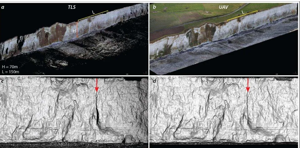
Figure 1 : Comparison of TLS vs UAV topographic coverage. Upper panel: colour point clouds of TLS (a) and UAV (b). Lower panel: topographic gradient of TLS (c) and UAV (d). UAV point cloud not only covers the strict object of interest (cliff face), but also the foreground and hinterland, which both are important to coastal risks managers. On the hinterland, it is possible to assess the amount of residual land that exists between cliff face and exposed assets. On the platform, remainders of cliff collapse lobes informs on the risk of outreach during a collapse.
Extracting the dense cloud represents the longest part of the process, attaining 350h for 1000 photographs at maximum resolution (24 Mpix). Processing was performed on a 40 cores windows server, 128 Go RAM but devoid of graphics card to speed up the processing as suggest by Agisoft. In the end, point clouds of 197Mpts for the winter campaign and 139 Mpts for the summer campaign described the cliff topography as well as its surrounding plateau and coastal platform at maximum photo resolution.
4. RESULTS
4.1 Qualitative comparison of TLS and UAV
Figure 1 represents the same cliff section measured by TLS and UAV. From this figure one sees that both TLS (ground based) and UAV (airborne) surveys covered pretty much the same surface area of cliff, during a single low tide (Figure 1). So both techniques performed equally well for the specific topic of interest: contributing to document cliff collapse hazard. Yet UAV surveys offer a much more complete view of the overall environment (Figure 1b). Not only was the cliff covered, but also the hinterland above the cliff and coastal platform below the cliff. If one is to grasp what controls cliff collapse and which effect a collapse will have on exposed assets (infrastructures, houses, cultivated fields as well as walkers on the coastal path and on the beach), UAV holds the capacity to document both questions. TLS only documents where rocks fell off the cliff and which shape properties they had. TLS does not tell coastal managers what it affected above and below.
A second aspect showed on Figure 1 concerns the faithfulness of relief description. While it makes no doubt today that TLS are outstanding tools for depicting landscape relief, the same is still doubted for structure-from-motion techniques. Figure 1
shows that the relief described in both surveys are qualitatively comparable. One may note that TLS survey was in fact less explicit in describing the cliff topography. An unfortunate shadow occurred behind a suspended rock mass, which passed unnoticed at the time of the survey, but created a hole in the point cloud. In comparison, because photo triggering rate was set to 1Hz and flight paths were carefully designed, the UAV-acquired point cloud did not suffer any shadow. It nevertheless shot a gigantic, highly redundant (far too redundant in fact) archive of photos. This proved computationally challenging with the available resources and begs for a more optimized shooting strategy.
Beyond these two remarks, the calibration defect of the TLS already alluded to, ruined any attempt of quantitative comparison, despite our best efforts to coin that question from the beginning.
4.2 Comparison of UAV surveys
Dewez et al., 2013 addressed the question of generating a meaningful rockfall inventory from repeated multiple-TLS-stations surveys. Among the hard point they came across, building a rigid reference frame for a multi-year repeated survey where permanent markers could not be established was a real challenge. Survey nails do not last in a platform covered by high tides twice a day. Because station-to-station co-registration was imperfectly achieved with respect to targets, whose position was not known with enough accuracy, reference frame rigidity was not fully achieved. They observed warping effects in the cliff topography from epoch to epoch and reduced them with a third degree polynomial fit for it behaved with an acceptable degree of tension.
Rigidity was then achieved to a level satisfactory to characterize rockfall object with a minimum representative volume of one litre (0.001m3) and significant differences of 26 to 36mm depending on the epoch compared. Although variable in The International Archives of the Photogrammetry, Remote Sensing and Spatial Information Sciences, Volume XLI-B5, 2016
absolute value, the detection threshold always retained the same level of statistical significance (p-value of 1/1000). Aware of this limitation, we explore whether SFM-generated relief can be safely considered rigid, and whether it may adversely affect rockfall inventories.
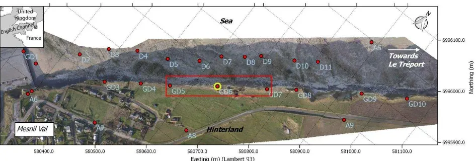
As TLS surveys were impacted by the positional quality of ground control points (GCP), we addressed the question to UAV point clouds in a similar manner. During both January (Figure 2) and June 2015, 30 GCP (black/white quadrants) were deployed in the field, with as optimal a distribution as could be
practically achieved with a planned deployment. Yet the same locations were not strictly reoccupied. Quadrants were made large enough (50x50cm² and 1x1m²) so that pin-pointing their centre was not an issue.
Here we explore the impact of the following question: what would be the consequence of removing just one GCP, located in the centre of the survey? And to establish the consequences, we compare the very same data set, January 2015, against itself (Figure 2).
Figure 2 : Orthophotography of Mesnil Val chalk cliff site from the UAV 27 January 2015 survey. Ground Control Points (GCP) location are symbolised in red point. Target GD6 in the centre is marked by a yellow circle. It is this GCP that was removed to test the rigidity of SFM-derived point clouds. High density point clouds are extracted from the red rectangle area.
One should note that GCP can be used for two purposes in Agisoft Photoscan: solving the block bundle adjustment (known to photogrammetrists as external orientation) and optionally simultaneously solving the self-calibration procedure (aka. camera internal orientation - function Optimize with appropriate camera parameters ticked). James and Robson (2014) asserted, with theoretical simulations and examples, that including oblique shots within the batch of photographs would take care of unresolved and unknowable camera internal orientation defects if the photos had all been shot parallel to one another. They noted that if oblique views could not be shot, which is often the case with fixed winged UAV, placing GCP in the central part of the survey was of paramount importance to avoid model doming. This doming was the signature of insufficiently resolved internal orientation (James and Robson, 2014). Three point clouds between GD5 and GD7 (Figure 2) were therefore prepared and compared. The reference point cloud of January 2015 (cloud 1) contains all GCP that served for exterior orientation as well as self-calibrating procedure. The second point cloud used all but one GCP (GCP GD6, see Figure 2), and the same camera calibration as cloud one (none of the camera calibration were ticked, camera calibration was set to fixed). The third point cloud had same GCP removed, but obtained a new calibration with this (n-1) GCP set. With this scheme, we isolate camera calibration effects from the GCP effects. Comparison of point cloud was performed under Cloud Compare v. 2.6.1 with algorithm M3C2 (Lague et al., 2013). By removing one GCP, we want to check whether the UAV point cloud remains rigid, and if not, check whether warping occurred because of the self-calibrating bundle adjustment (improved or worsened calibration) or whether the GCP itself warped the topographic result.
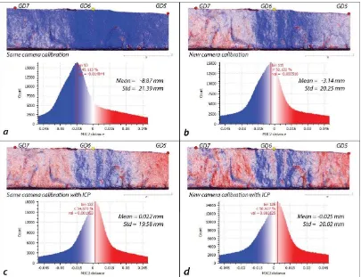
Difference maps (Figure 3) show that both clouds where one GCP GD6 was withdrawn from the orientation solution were affected. The effect is most severe when a unique calibration is used (Figure 3a). The median difference is -14mm (Figure 3a) as opposed to -3mm (Figure 3b) and the width of the area affected is much broader (more than 200m, as opposed to a more local bump of 90m-wide). The amplitude of the bump reaches 20 mm.
The difference pattern between cloud 2 and cloud 1 looks as if a simple cloud translation may have occurred. To test this possibility, an Iterative Closest Point (ICP) alignment was then applied. ICP alignment determines the most likely 6 parameters transformation to reconcile two point clouds (here, the scale parameter was kept constant). Unsurprisingly, M3C2 differences between aligned clouds reduced to nearly 0 after applying a, ICP fine registration, ICP played its role in determining the appropriate translation in the cliff-normal direction. But what is also apparent is the warping affecting on both self-calibrated and fixed calibration clouds. The difference pattern of both clouds is very similar. The warping affects a 90-m-wide area. ICP did not solve a vertical offset which is visible on rock mass ledges (L shape on the left of the test area and rectangle on the right, two-third up the cliff). From this experiment, we conclude that GCP number and placement have a strong influence on the model geometry. Removing one GCP can throw a geometry by 2cm (20mm) or so between remaining GCP spaced by 240m.
This amplitude bias may seem little, but it should be related to the original purpose of this paper: quantifying rockfall hazard. Small rockfalls occur far more frequently than larger rockfall, the relationship being controlled by a power-law (e.g. Dewez et al. 2013). To establish an empirical probabilistic rockfall hazard relationship on a set of representative rockfall magnitudes, in a matter of a few years to be practical for rockfall risk managers, The International Archives of the Photogrammetry, Remote Sensing and Spatial Information Sciences, Volume XLI-B5, 2016
capturing small rockfalls is paramount because they occur often enough to be seen rapidly. The inventory of Dewez et al. (2013) was deemed complete for events comprised between 10-3 and 102 m3. Larger events occurred by chance during the total span of 2.5 years. Smaller rockfalls were occasionally missed probably because of the limit of cliff relief resolution. The rockfall scar detection threshold of the case study described by Dewez et al. (2013) was comprised between 26 and 36 mm. The equivalent statistical threshold (quantile at 99.9% of observed differences) extracted from the gaussian distribution reported in Figure 3c and 3d come as 62mm (case with self-calibration) and 61mm (case with same calibration).
From this discussion it appears that for rockfall applications, one cannot tolerate an artificial bias of 20mm solely for poorly constrained reasons. And what if it were used nevertheless? What would be the minimum rock volume which would not be detected?
Answering this question is tricky. Let us turn it the other way around. From the empirical probabilistic power-law relationship (Dewez et al., 2013), the event volume expected to occur twice every day per kilometre of cliff is 0.013m3. This volume is a block of 325mm x 400mm x 100mm. Despite a possible 20mm bias, this signal will come above the noise level, as the thickness is well above the 62mm detection threshold and concerns a coherent patch of at least 450 points (considering point density of 1pt/17mm). At Mesnil Val, without further geometric adjustments, the performed UAV survey is capable of producing a rock scar data set recognizing the twice-daily rockfall event.
Why rigidity is not achieved when removing one GCP is unclear. We were aware of this possibility and had applied
James and Robson’s (2014) recommendations for that very purpose: oblique views and enough GCPs as was standard in the old days of analogic photogrammetry. Even though three flight paths with different aiming direction (horizontal, 45°oblique and vertical) were designed to limit doming, it occurred. There is a possibility that the number of parallel-viewing photo pairs overwhelmed the number of oblique photo pairs, and thus dwarfed their compensating effect.
A possible improvement for the future is to perform a camera calibration flight before the survey itself, and assume that this calibration can apply. In this way, self-calibration would be performed on a tighter terrain, more densely covered with GCP, independently of the cliff site orientation itself. This will however pose a series of other logistical problems. Self-calibrating bundle adjustments were a great progress two decades back. But are they really applicable to the level of precision desired here? Accurate GCP comes back to being of paramount importance.
At present the processing alternative we will chose is to perform a piecewise ICP adjustment for cliff portions of a set length e.g. about one quarter of the spacing between GCP above and below the cliff. Here the wavelength of the landward doming is ca. 100m for GCP distant by 240m. The obvious limitation of this is that for diachronic cliff faces, rockfalls will have occurred and topography will have changed. Comparing two epochs with a fine alignment step using observed topography and avoiding biases will prove intrinsically tricky and defeat the purpose and necessity of a rigid reference frame.
Figure 3 : Comparison between January point cloud (cloud 1) with all the GCP and variation of the same point cloud a. Same Camera calibration and GD6 GCP removed (cloud 2) . b. New Camera calibration and GD6 GCP
removed (cloud 3). c. The cloud 2 with ICP transformation applied on the cloud 1. d. The cloud 3 with ICP transformation applied on the cloud 1.
4.3 Quantitative comparison of TLS and UAV
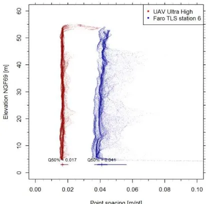
The literature, and first intuition, has questioned the capability of structure-from-motion (SFM) techniques to match the point density of lidar measurements. This paper is no exception. TLS works with a fixed scanning increment which intersects a surface at increasing spacing as obliquity and distance increase. At Mesnil Val, we show that Photoscan point clouds extracted at ultra-high density are not only denser than measurements with the Faro330 TLS but spatial sampling was constant over the entire cliff height (Figure 5). Median point spacing achieved with SFM is 17mm, while only 41mm for TLS and worsening with height (Figure 5).
One could question the reason for extracting a cloud with such point density. Here is why. After having run topographic comparisons between SFM point clouds at difference resolutions, peculiar features stood out. At lower density, point clouds described cliff topography with a lesser degree of
faithfulness. Chalk bed edges would disappear, for instance. This is not surprising. But changing point density also fills in depressions and shaves off the crests over breadths of several meters wide, which is much wider than point spacing (Figure 4)
The message we retain from this rapid description is that because depressions are filled in and crests shaved off, ghost volumes related to processing algorithms will occur. And what is worse for rockfall mapping application is that these ghost topographies locate themselves precisely where the signal will be sought after. Prominent bed edges are places where rock will fall first. If topography cannot be trusted in those places, then building inventories with this technique is worthless. Choosing the highest resolution is the only option to describe the best possible topography and limit artefacts. This conclusion is actually detrimental for rockfall mapping applications as the highest point cloud density is the most computationally intensive, sometimes prohibitively so.
Figure 4 : Effect of decreasing point cloud density in Photoscan. Three reduced resolutions (High, Medium, Low) are compared with the densest possible model (Ultra-High). It turns out that topography is expectedly smoothed with lower densities along sharp edges, but a zebra-skin effect appears on either sides of sharp gradients.
Figure 5 : Comparison of point cloud density variation with cliff height between UAV and TLS point cloud. UAV point density stays constant with
cliff height (median = 17 mm between adjacent points) while TLS point cloud has a median density of 41mm but varies with height.
5. CONCLUSION
Topographic measurements of Mesnil-Val cliffs with UAV provided a fast means of acquisition, making it possible to survey a 50-60ha site including the cliff face as well as the coastal platform and its hinterland. The geometry described by 3D point clouds extracted by Structure-from-Motion techniques is close to that described with Terrestrial Laser Scanners (TLS). SFM point clouds, just like TLS point clouds, are not rigid objects because of the piecewise construction of the dataset. Removing one ground control point from the overall orientation may cause local model distortion, despite acquiring oblique views to limit this effect, as recommended in the literature. Admittedly, these deformation may be modest in amplitude (here it reached -14mm in the worst case), but this is a bias which will affect the sensitivity of rockfall scars extraction and the overall sensitivity of the rock scar inventory.
Compared to TLS data, SFM point cloud density is both denser and more uniform over the entire cliff height. And comparison between different SFM point cloud densities shows that The International Archives of the Photogrammetry, Remote Sensing and Spatial Information Sciences, Volume XLI-B5, 2016
reducing the density not only produces a coarser relief definition, but also creates topographic modifications: crests are shaved off and depressions are filled in over a spatial wavelength much broader than point density reduction would let suspect. Because these topographic features are where rock scars do locate, it is absolutely not desirable to reduce point cloud density, despite the strong impact high image resolution has on computation time.
Finally, UAV surveys, in the Mesnil Val case study, seem fit to resolve the expected twice-daily rockfall event of 0.013m3 for every cliff kilometre. They thus prove very useful to survey larger areas than terrestrial laser surveys in particular for sites where access is very limited in time (e.g. tidal beaches) or inaccessible from the ground (mountainous areas). The ratio productivity / cost of UAV surveys is superior to other topographic measurement techniques for accuracy possibly lower but acceptable in terms of their performance.
ACKNOWLEDGEMENTS (OPTIONAL)
We thank Dimitri Lague from Geoscience Rennes for lending us the FARO330 TLS for the purpose of this project. Personnel costs (TD & JL) to achieve this project were funded by ANR-Carnot-Investissement d’Avenir Captiven project. TD benefited from a mobility grant from Institut Carnot BRGM that funded the time during which this paper was written.
REFERENCES
Abellán, A., Calvet, J., Vilaplana, J.M., Blanchard, J., 2010. Detection and spatial prediction of rockfalls by means of terrestrial laser scanner monitoring. Geomorphology 119, 162– 171. doi:10.1016/j.geomorph.2010.03.016
Costa, S., Delahaye, D., Freire-Diaz, S., Di Nocera, L., Davidson, R., Plessis, E., 2004. Quantification of the Normandy and Picardy chalk cliff retreat by photogrammetric analysis. Geol. Soc. London, Eng. Geol. Spec. Publ. 20, 139–148. doi:10.1144/GSL.ENG.2004.020.01.11
Dewez, T., Gebrayel, D., Lhomme, D., Robin, Y., 2009. Quantification de l’évolution des côtes sableuses et rocheuses par photogrammétrie et lasergrammétrie. La Houille Blanche 32–37.
Dewez, T.J.B.,, Rohmer, J., Regard, V., and Cnudde, C., 2013. Probabilistic coastal cliff collapse hazard from repeated terrestrial laser surveys: case study from Mesnil Val (Normandy, northern France), Journ. Coast. Res., Sp. Iss. 65, DOI:10.2112/SI65-119
Dewez, T.J.B., Rohmer, J., Closset, L., 2007. Laser survey and mechanical modelling of chalky sea cliff collapse in Normandy, France, in: Proceedings of the International Conference on Landslides and Climate Changes, Ventnor, England. pp. 281– 288.
Lasseur, E., Guillocheau, F., Robin, C., Hanot, F., Vaslet, D., Coueffe, R., and Neraudeau, D., 2009, A relative water-depth model for the Normandy Chalk (Cenomanian– Middle Coniacian, Paris Basin, France) based on facies patterns of metre-scale cycles: Sedim. Geol., v. 213, no. 1-2, p. 1–26, doi: 10.1016/j.sedgeo.2008.10.007.
James, M.R., Robson, S., 2014. Mitigating systematic error in topographic models derived from UAV and ground-based image networks. Earth Surf. Process. Landforms 39, 1413– 1420. doi:10.1002/esp.3609
James, M.R., Robson, S., 2012. Straightforward reconstruction of 3D surfaces and topography with a camera: Accuracy and geoscience application. J. Geophys. Res. Earth Surf. 117, n/a– n/a. doi:10.1029/2011JF002289
Lague, D., Brodu, N., Leroux, J., 2013. Accurate 3D comparison of complex topography with terrestrial laser scanner: Application to the Rangitikei canyon (N-Z). ISPRS J. Photogramm. Remote Sens. 82, 10–26. doi:10.1016/j.isprsjprs.2013.04.009
Lasseur, E., Guillocheau, F., Robin, C., Hanot, F., Vaslet, D., Coueffe, R., and Neraudeau, D., 2009, A relative water-depth model for the Normandy Chalk (Cenomanian–Middle Coniacian, Paris Basin, France) based on facies patterns of metre-scale cycles: Sedimentary Geology, v. 213, no. 1-2, p. 1– 26, doi: 10.1016/j.sedgeo.2008.10.007.
Regard, V., Dewez, T., Bourles, D.L., Anderson, R.S., Duperret, A., Costa, S., Leanni, L., Lasseur, E., Pedoja, K., Maillet, G.M., 2012. Late Holocene seacliff retreat recorded by 10Be profiles across a coastal platform: Theory and example from the English Channel. Quat. Geochronol. 11, 87–97. doi:10.1016/j.quageo.2012.02.027
Rohmer, J., Dewez, T., 2015. Analysing the spatial patterns of erosion scars using point process theory at the coastal chalk cliff of Mesnil-Val, Normandy, northern France. Nat. Hazards Earth Syst. Sci 15, 349–362. doi:10.5194/nhess-15-349-2015
Rosser, N.J., Brain, M.J., Petley, D.N., Lim, M., 2014. Citation for published item: Coastline retreat via progressive failure of rocky coastal cliffs. doi:10.1130/G34371.1
Senfaute, G., Amitrano, D., Lenhard, F., Morel, J., Gourry, J.C., 2005. Etude experimentale en laboratoire de l’endommagement des roches de craie par methode acoustique et correlation avec des resultats in-situ. Rev. Française Géotechnique, Press.
Senfaute, G., Duperret, A., Lawrence, J.A., 2009. Micro-seismic precursory cracks prior to rock-fall on coastal chalk cliffs: a case study at Mesnil-Val, Normandie, NW France. Nat. Hazards Earth Syst. Sci 9, 1625–1641.