isprsarchives XXXIX B3 205 2012

GENERAL MATHEMATICAL MODEL OF LEAST SQUARES 3D SURFACE

MATCHING AND ITS APPLICATION OF STRIP ADJUSTMENT

Z. Q. Zuo a, *, Z. J. Liu a, L. Zhang a, S. Tuermer b

a

Chinese Academy of Surveying and Mapping, 28, Lianhuachixi Road, Haidian District, Beijing, P.R. China 100830-

(zqzuo, zjliu, zhangl)@casm.ac.cn

b

Remote Sensing Technology Institute (IMF), German Aerospace Center (DLR), Oberpfaffenhofen, Germany-

sebastian.tuermer@dlr.de

Commission III, WG III/2

KEY WORDS: 3D surface matching, 3D similarity transformation, strip adjustment, laser altimetry ABSTRACT:

Systematic errors in point clouds acquired by airborne laser scanners, photogrammetric methods or other 3D measurement techniques need to be estimated and removed by adjustment procedures. The proposed method estimates the transformation parameters between reference surface and registration surface using a mathematical adjustment model. 3D surface matching is an extension of 2D least squares image matching. The estimation model is a typical Gauss-Markoff model and the goal is minimizing the sum of squares of the Euclidean distances between the contiguous surfaces. Besides the generic mathematical model, we also propose a concept of conjugate points rules which are suitable for special registering applications, and compare it to three typical conjugate points rules. Finally, we explain how this method can be used for the registration of real 3D point sets and show co-registration results based on airborne laser scanner data. Concluding results of our experiment suggest that the proposed method has a good performance of 3D surface matching, and the least normal distance rule returns the best result for the strip adjustment of airborne laser altimetry data.

2.1

* Corresponding author

1. INTRODUCTION

A laser scanner system consists of three main components: GPS, IMU and Laser unit. Data collection is carried out in a strip-wise form and the object coordinates of the laser footprints are determined using the direct geo-referencing from the GPS/IMU. Due to the systematic errors in the laser scanner components or in the alignment, adjacent strips usually have discrepancies. Such discrepancies are serious to the terrain modeling and object reconstruction. So the most emphasis of our approach is to find a general solution for the registration problem in 3D modeling.

In the field of Computer Vision, one of the most famous methods is the Iterative Closest Point (ICP) algorithm proposed by Besl and McKay (1992), Chen and Medioni (1992), and Zhang (1994). And in the field of LiDAR and photogrammetry, people use data driven methods to do strip adjustment. The purpose of data driven methods is establishing a 3D transformation between two point sets, which represent an irregular spatial sampling of the same surface (Shan, 2008). The earliest data driven methods, only consider the difference on elevation between strips, using linear system parameters with conjugate points of adjacent strips (Crombaghs, 2000; Kornus and Ruiz, 2003). And then Kilian (1996) uses a 12 parameters model to replace the linear parameters. In order to eliminate the strong correlation of the 12 parameters model, Vosselman and Maas (2001) use a 9 parameters model to estimate 3D transformation. Morin and El-Sheimy (2001) just considered the global translation and rotation transformation to establish a 6 parameters model. And if the scale factor can be involved, the 7 parameters of a space similarity transformation model may return an effective solution for the strip adjustment (Robert, 2004; Gruen and Akca, 2005).

T

Least squares 3D surface matching (LS3D) is a typical data driven method, where the sum of squares of the Euclidean distances between the neighboring surfaces is minimized. LS3D has many advantages compared with the ICP method,

and the significant one is that conjugate points of LS3D can be obtained using interpolation on 3D surface but ICP needs real points. Hence, LS3D can achieve higher accuracy in many cases, especially in the co-registration routine of different resolution point clouds.

In this approach, we propose a mathematical model for LS3D. It is a general model for estimating orthomorphic transformation parameters for conjugate surfaces. Three different searching rules of conjugate points on adjacent surfaces are defined in this adjustment system and each rule can be well used in the new estimate model. Also the differences are compared to existing methods and are shown in detail. At last, two groups of real airborne laser scanner data are used to show the capabilities of our method.

2. 3D SURFACE MATCHING

New Estimation Model

The major task of 3D surface matching is finding the transformation parameters between template surface

and searching surface . The

overlapping area between two surfaces is , which

can be defined as

O

F

estimation of the orthomorphic transformation parameters is as follows:

( , , )

{ ( , , )}

G x y z

=

T F x y z

(1) To express the geometric relationship between the conjugate surfaces, a seven parameters similarity transformation is used:

'

where

( , , )

x y z

∈

F

,

( ', ', ')

x y z

∈

G

,

R

( , , )

ϕ ω κ

is

the orthogonal rotation matrix,

[ ,

is the translation

vector, and m is the scale factor.

, ]

T

x y z

t t t

In order to perform least squares estimation, the true error vector is introduced to describe the discrepancy between the conjugate surfaces:

( , , )

V x y z

( , , )

( , , )

( , , )

V x y z

=

G x y z

−

F x y z

(3) As continuous 3D surfaces have to be sampled with discrete coordinates, a 3D surface matching is automatically translated into a registration of point clouds. So the true error vector of equation (3) can be approximately expressed with the Euclidean distance of conjugate points, and the aim of least squares estimation is defined as follows:

||

dd

||

=

min

∑

(4) If the square of the distance is set to , the new mathematical model of 3D surface matching can be simply defined as follows:

Since equation (5) is nonlinear, it must be linearized by the Taylor expansion, ignoring 2nd and higher order terms.

0 x y

where can be considered as residual of the Taylor expansion, and the Euclidean distance of conjugate points will be set to zero at the end of the LS3D routine. Hence, the observation error equation can be simplified as:

V

The matrix form of equation (7) is as follows:

,

V

=

AX

+

L

P

(8)

where

A

is the design matrix,

is the parameter vector, and

is the constant vector that consists of the Euclidean

distances between the template and searching surface elements, is the weight matrix of the error observation vector.

[ , , , , , , ]

_{x y z} T

X

=

t t t

ϕ ω κ

m

0

L

=

D

P

The distribution of the random variable is

, with the statistical expectation

, (8) is a typical Gauss-Markoff estimation model. In order to control the estimation quality, an additional error observation vector of the unknown parameters could be imported (Robert,2004; Gruen and Akca, 2005).

,

e e

V

=

IX

+

L

P

_e (9)

Where

I

is the identity matrix, and is the constant vector of the error equation, is a priori weight matrix of unknown

parameters. If zero weight

((

is set, the i-th

parameter is assigned as free variable, and if an infinite weight

value constant. Combining equation (8) and equation (9), the maximum likelihood solution of unknown parameters can be estimated as follows:

σ

is the mean square error of the weighted units of the observations,

n

is the number of error observation equations, and

u

is the number of unknown parameters,

r

= −

n u

are the components of abundant observation.

2.2 Conjugate Points Rules

Since it is rather difficult to locate feature points in a local window on 3D surfaces, how to establish the conjugate points between 3D overlapping regions, is the core strategy in the 3D surface matching procedure. In our method, the conjugate points rule is unlimited. We could define some new rules for specified applications, because the mathematical model of the adjustment, defined in 2.1, is generic for available rules. And, it is the major advantages of our proposed method compared with existing methods.

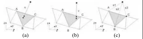
In this section, we list three strategies for establishing conjug-ate points on 3D surfaces. The first definition called LND rule is the same as the Least Normal Distance method (Robert, 2004; Gruen and Akca, 2005), using pedal point of triangle in normal direction. The second definition called LZD rule is the same as the Least Z-Difference method (Rosenholm, 1988), using the intersection point of a triangle in vertical direction. The last definition called ICP rule is the same as the Iterative Closest Point method (Besl and McKay, 1992), using two, the closest points in the entire point sets as conjugate points. With the 3D surface representation of triangulated irregular network structure, the conjugate point rules can be listed as follows:

(a) (b) (c)

Figure 1. Conjugate points definitions for surface matching with TIN structure: (a) LND rule, (b) LZD rule, (c) ICP rule.

where

A

B

and are the 3 vertexes of the candidate conjugate region on the searching surface, and

n

is the normal vector of the located triangle,

v

is the vertical vector of the located triangle, are behalf of the Euclidean

distances from the interpolation point to the 3 vertexes, and the

C

1

s

s

₂

s

₃

closest point is the conjugate point in

Figure 1(c).

3

min{ ,

1 2

, }

s

=

s s

s

₃

2.3 Precision and Reliability

Precision and reliability are the two basic factors for quality analysis of adjustment systems. The theoretical precision of unknown parameters and the correlation coefficient matrix are also an important basis for the procedure of least squares

solution (Li and Yuan, 2002). The theoretical precision

σ

_i and the correlation coefficient can be estimated from a co-factor matrix of unknown parameters.

0

To detect the gross error of the observation, a simple and efficient weight function is used in our robust estimation routine.

In equation (15), when the gross observed value is detected, its

weight will be set to zero , in other case, the weight of

the observed value will be set to one . In our

experiment, when the constant

0

adjustment system has a good performance to estimate the unknown parameters.

2.4

z

Compared with Existing Methods

The procedure of LS3D proposed above is separated into two parts, the adjustment model and the conjugate points rule. The adjustment model can be derived form the formula of the Euclidean distance. So, it is easy to adapt to new conjugate points rules and good for some special applications. In this section, we show the differences between our method and existing methods.

·compared with Gruen’s method

The most important factors for adjustment process are the coefficient items and constant item of the error equation. Gruen and Akca (2005) derived the error coefficients under certain assumptions and lacking of rigorous mathematical formula. They proposed that the vector

[

∂ ∂ ∂ ∂ ∂ ∂

D

/

t

_x

,

D

/

t

_y

,

D

/

t

]

T is only related with the coefficients of a local triangle plane. Hence, if the matching point does locate the same triangle, the vector values are constant. But under the rigorous derivation of our formula, the

vector

[

∂ ∂ ∂ ∂ ∂ ∂

D

/

t

_x

,

D

/

t

_y

,

D

/

t

_z

]

T may be changed, even if the local triangle has not changed during the iteration procedure and the vector values are related with the three coordinate components of current conjugate points. Another difference is the constant item of error equation. In Gruen’s method, they define the conjugate points distance as constant item directly, but we use the square value because of the smaller amount of computation. Especially, we found Gruen’s method maybe need quite good approximations and we are less after similar iteration times, under the same priori weights of the unknown parameters.

·compared with ICP method

ICP method is a linear squares solution for estimation of the 6-parameters between two point sets. So, ICP needs a relatively

high number of iterations in some tests (Pottmann et al. 2004). Another difference is that conjugate points of LS3D can be obtained using interpolation on a 3D surface but ICP needs real points. So LS3D can achieve higher accuracy in many cases, especially in the co-registration routine of different resolution point clouds.

·compared with Rosenholm’s method

Rosenholm’s adjustment model can be considered as the special form of our approach. If we define the conjugate points as Figure 1(c), the equation (5) can be derived to

, which is the same as Rosenholm’s model. In many cases, the registration accuracy of this model is limited, because it can only meet the discrepancy in z direction of two point sets.

2

(

'

D

= −

z

z

)

3. LS3D AND STRIP ADJUSTMENT

Strip adjustment is a relevant problem for the post-processing of airborne laser scanner data. 3D surface matching is a typical data-driven method of strip adjustment. The transformation parameters of the adjacent strips can be estimated by a least squares routine. Each strip can be seen as a single surface, and the conjugate points can be interpolated by one of the finite element methods discussed in section 2.2.

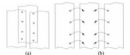
(a) (b)

Figure 2. Surface matching for laser scanning strips: (a) overlapping area on conjugate surfaces, (b) Estimating transformation parameters with conjugate points.

In this work, we are aimed to use primitives, which can be derived with minimal pre-processing of the original laser scanner point clouds. To satisfy the 3D surface matching procedure, we chose one strip of the original points, while the other strip is represented by a triangulated irregular network (TIN).

Figure 3. Interpolation of conjugate points between template surface and searching surface in LS3D routine.

In Figure 3,

q

can be interpolated by the vertex coordinates of local finite elements in

Tri A B C

( , , )

.

4. EXPERIMENT RESULTS

Two practical examples are given to show the capabilities of our proposed method. All experiments were carried out using software based on C code that runs on a MS Windows operating system. In order to increase the accuracy of conjugate points between adjacent strips, it is necessary to label terrain points and off-terrain points by a fast filtering

0 0 0

0.0

x y y

t

=

t

=

t

=

_{0 0 0}

0.0

technology. And the initial approximation of seven unknown parameters is used as:

,

ϕ ω κ

=

= =

,

m

₀

=

1.0

In the iteration routine of the least squares solution, the convergence of rotated angles can be set as 1e-6 (rad) or 1e-7 (rad), and the number of iterations may be less than 20.

4.1 Data Description

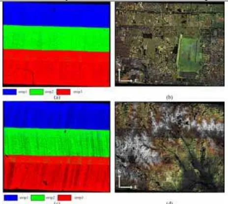
Two typical data sets were selected in this section. The scanning data from Hebei and Henan province, China was received by an ALS60 (Leica Geosystems) airborne laser scanner at 1000 meters above the ground. The Hebei data set is an urban scene, including buildings, roads, trees, rivers, etc. and the Henan data set is a mountainous area, including terraced field, scarps, isolated trees and a few low buildings.

Figure 4. Two groups of LiDAR raw data sets: (a)~(b) Hebei data set of urban scene, (c)~(d) Henan data set of mountainous area.

Some other quantitative information of our experiment data sets can be seen in table 1.

Table 1. Properties of the test data sets

The purpose of this section is to show 2 categories of results from our proposed method: profiles registering, estimating results and accuracy assessment of unknown parameters. Profile results are shown in figure 5. Estimating results of unknown parameters are listed in table 2 and the corresponding accuracy assessments are in table 3.

4.2 Results

All of the results show that the LS3D proposed in our approach can achieve the transform parameters between two overlapping

surfaces, and the conjugate points rule plays an important role in the LS3D procedure.

5. CONCLUSIONS

A general mathematical model for co-registration of two 3D surfaces is presented. Our proposed method, estimates the transformation parameters between reference surface and registration surface, using the generalized Gauss Markoff model which is a well-known method in geodesy and photogrammetry. Our mathematical adjustment model is generic to effective conjugate point rules. In this paper, there are three definitions of conjugate points presented and described. Finally, the LND definition shows the highest precision in the experiments of surface matching or strip adjustment.

At last, the derived conclusions may be the following ones. Due to the influence of multiple echo points in laser scanner data, it is necessary to remove height anomaly points and irregular geometric shapes, e.g. tree points, using fast filtering technology or rough classification routines. These points discussed above can reduce the co-registration accuracy. Another important issue is that if there are not enough geometric features or enough overlap between conjugate surfaces, the iteration will fail. In this case, we can add some roof points to strengthen geometric constraints between surfaces.

REFERENCE

Ackermann, F., 1984. Digital image correlation: performance and potential application in photogrammetry. Photogrammetric Record, 11(64), pp. 429-439.

Besl, P.J., and McKay, N.D., 1992. A method for registration of 3D shapes. IEEE Transactions on Pattern Analysis and Machine Intelligence, 14(2),pp. 239-256.

Crombaghs, M.J.E., Brugelmann, R.,2000. On the adjustment of overlapping strips of laser altimeter height data. International Archives of Photogrammetry and Remote Sensing, 33(B3), pp.224-231.

Chen, Y., and Medioni, G., 1992. Object modelling by registra-tion of multiple range images. Image and Vision Computing, 10(3), pp. 145-155.

Gruen, A., 1984. Adaptive least squares correlation – concept and first results. Intermediate Research Project Report to Heleva Associates, Inc., Ohio State University, Columbus, Ohio, March, pp. 1-13.

Gruen, A., 1985a. Adaptive least squares correlation: a power-ful image matching technique. South African Journal of Photogrammetry, Remote Sensing and Cartography, 14(3), pp. 175-187.

Gruen, A., and Akca D., 2005. Least squares 3D surface and curve matching. ISPRS Journal of Photogrammetry and Remo-te Sensing 59(3), pp.151-174.

Kornus, W., Ruiz, A. 2003. Strip adjustment of LiDAR data. International Archives of Photogrammetry and Remote Sensing, 33(3/W), pp.47-50.

Kilian, J., Haala, N., Englich, M., 1996. Capture and evaluation of airborne laser scanner data. Internatio-nal Archives of Photogrammetry and Remote Sensing, 31(B3), pp.383-388. Li, D.R., and Yuan, X.X., 2002. Error Processing and Reliabi-lity Theory. Wuhan University, China, pp.92-120.

Maas, H.G., 2000. Least-Squares matching with airborne laser scanning data in a TIN structure. International Archives of Photogrammetry and Remote Sensing, 33(3A), pp. 548-555. Morin,K. and El-Sheimy, N., 2002. Post-mission adjustment of airborne laser scanning data, Proceedings XXII FIG International Congress, Washington, DC, April 19-26, 12 pp., CD-ROM. Pottmann, H., Leopoldseder, S., and Hofer, M., 2004. Registration without ICP. Computer Vision and Image Understanding, 95(1),pp. 54-71.

Pertl, A., 1984. Digital image correlation with the analytical plotter planicomp C-100. International Archives of Photogra-mmetry and Remote Sensing, 25(3B),pp.874-882.

Rosenholm, D., 1988. Three dimesional absolute orientation of stereo models using digital elevation models. Photogrammetric Engineering and Remote Sensing, 54(3),pp 1385-1389. Robert, M. P., 2004. Theory and application of weighted least squares surface matching for accurate spatial data registration. Australia: The University of Newcastle:15-30.

Shan, J., Toth, C.K., 2008. Topographic laser ranging and scanning: principles and processing. Boca Raton: CRC Press.

Vosselman, G., Maas, H.G.,2001. Adjustment and filtering of raw laser altimetry data, Proceedings OEEPE Workshop on Airborne Laserscanning and Interferometric SAR for Detailed Elevation Models. OEEPE Publications No.40,pp.62-72.

Zhang, Z., 1994. Iterative point matching for registration of free-form curves and surfaces. International Journal of Computer Vision, 13(2), pp. 119-152.

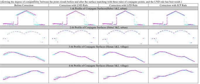
Figure 5. Profiles in overlapping strips

(showing the degree of compatibility between the point clouds before and after the surface matching with three rules of conjugate points, and the LND rule has best result.)

Before Correction Correction with LND Rule Correction with LZD Rule Correction with ICP Rule

1-th Profile of Conjugate Surfaces(Hebei 1&2, urban)

2-th Profile of Conjugate Surfaces (Hebei 3&2, urban)

3-th Profile of Conjugate Surfaces (Henan 1&2, village)

4-th Profile of Conjugate Surfaces (Henan 3&2, village)

Table 2. Estimated results of unknown parameters between conjugate surfaces.

(Iteration number and calculation times are listed in Table 2, and the time and iteration number are similar for three rules because of using same adjustment model. )

data set strip NO.

overlap number

(1.0e+05) iteration

time (sec)

tx

(m)

ty

(m)

tz

(m)

ϕ

(deg)

ω

(deg) (deg)

κ

m

LND Rule

hebei 1&2 203.45 18 108 -0.586 1.799 -3.345 0.00059 0.0670 0.0056 0.99997

hebei 3&2 199.34 15 95 0.238 0.461 -0.364 0.0024 0.0127 0.0097 0.99978

henan 1&2 189.24 17 102 -1.960 3.614 -3.226 0.00085 0.0780 -0.0023 1.000046

henan 3&2 186.74 13 82 -2.275 1.911 -1.334 0.00014 0.0320 -0.0052 0.99998

LZD Rule

hebei 1&2 203.45 15 99 -0.504 1.933 -3.277 0.00047 0.0690 0.0063 0.99999

hebei 3&2 199.34 13 78 0.394 0.577 -0.240 0.0064 0.0178 0.0067 0.99963

henan 1&2 189.24 14 85 -1.798 3.668 -3.104 0.00358 0.0808 -0.0010 1.000062

henan 3&2 186.74 15 88 -2.221 1.983 -1.152 -0.00002 0.0320 -0.0036 0.99991

ICP Rule

hebei 1&2 203.45 17 103 -0.578 1.892 -3.278 0.0021 0.0675 0.0078 0.99994

hebei 3&2 199.34 17 94 0.334 0.533 -0.172 0.0038 0.0148 0.0101 0.99983

henan 1&2 189.24 16 93 -1.904 3.779 -3.034 0.0023 0.0810 0.0005 1.000076

henan 3&2 186.74 15 85 -2.109 1.998 -1.256 0.0019 0.0347 -0.0047 1.000023

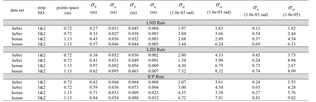
Table 3. Accuracy assessment for least squares 3D surface matching.

(Theoretical accuracy and error of unit weight are listed in table 3 and the LND rule has best accuracy.)

data set strip NO.

points space (m)

0

σ

(m)

tx

σ

(m)

ty

σ

(m)

tz

σ

(m)

ϕ

σ

(1.0e-03 rad)

ω

σ

(1.0e-03 rad)

σ

κ (1.0e-03 rad)

m

σ

(1.0e-05)

LND Rule

hebei 1&2 0.72 0.27 0.031 0.045 0.004 1.97 1.83 0.12 1.02

hebei

3&2 0.72 0.33 0.027 0.038 0.003 2.04 3.66 0.54 2.44

henan 1&2 1.13 0.43 0.036 0.032 0.003 2.68 2.89 0.37 4.54

henan 3&2 1.13 0.57 0.046 0.044 0.005 3.44 6.24 0.69 6.33

LZD Rule

hebei 1&2 0.72 0.38 0.052 0.030 0.002 2.80 4.33 0.45 3.73

hebei

3&2 0.72 0.41 0.031 0.049 0.001 1.54 5.90 0.24 8.94

henan 1&2 1.13 0.97 0.082 0.056 0.009 4.30 6.79 0.73 2.67

henan 3&2 1.13 0.62 0.095 0.063 0.007 7.32 8.32 0.74 8.09

ICP Rule

hebei 1&2 0.72 0.42 0.044 0.064 0.008 3.07 3.61 0.24 1.55

hebei

3&2 0.72 0.59 0.036 0.073 0.004 3.00 4.54 0.03 4.28

henan 1&2 1.13 0.71 0.033 0.069 0.023 4.35 3.38 0.27 5.76

henan 3&2 1.13 0.84 0.054 0.088 0.012 6.72 7.91 0.83 9.02