PERFORMING IMPROVED TWO-STEP CAMERA CALIBRATION WITH WEIGHTED
TOTAL LEAST-SQUARES
J. Lu a a
Dept. of Surveying and Geo-informatics, Tongji University, Shanghai – [email protected]
Youth Forum
KEY WORDS: camera calibration; two-step method; lens distortion; Errors-In-Variables (EIV) model; Weighted Total
Least-Squares (WTLS); Gauss-Helmert model
ABSTRACT:
In order to improve the Tsai’s two-step camera calibration method, we present a camera model which accounts for major sources of lens distortion, namely: radial, decentering, and thin prism distortions. The coordinates of principle points will be calculated at the same time. In the camera calibration model, considering the errors existing both in the observation vector and the coefficient matrix, the Total Least-Squares (TLS) solution is preferred to be utilized. The Errors-In-Variables (EIV) model will be adjusted by the solution within the nonlinear Gauss-Helmert (GH) model here. At the end of the contribution, the real experiment is investigated to demonstrate the improved two-step camera calibration method proposed in this paper. The results show that using the iteratively linearized GH model to solve this proposed method, the camera calibration parameters will be more stable and accurate, and the calculation can be preceded regardless of whether the variance covariance matrices are full or diagonal.
1. INTRODUCTION
Because actual cameras are not perfect and sustain a variety of aberrations, the relationship between object space and image space cannot be described perfectly by a perspective transformation. Digital camera calibration is the process of determining the interior and/or the exterior orientation parameters of the camera frame relative to a certain world coordinate system.
The techniques for camera calibration can be mainly classified into three categories (Juyang Wenig et al., 1992): 1) Direct Nonlinear Minimization (Brown, 1966; Wong, 1975; Faig, 1975); 2) “Closed-Form Solution” (Wong, 1975; Ganapathy, 1984; Faugeras and G. Toscani, 1986). 3) “The Two-step Method” (Tsai, 1987).
The two-step method is suitable for most calibration problems, and the iterative convergence speed is fast, since the number of parameters to be estimated through iterations is relatively small. However, this method can only deal with radial distortion and cannot be extended to other types of distortion (Wenig et al., 1992).
The Least-Squares (LS) adjustment within the Gauss-Markov (GM) model is usually used to calculate the calibration parameters from a redundant set of equations (y e y Ax). LS estimation is the best linear unbiased estimation when the error vectoreyin observation vectoryis normally distributed, and the
matrix of variablesAis error-free.
However, camera calibration, various random errors may bring inaccuracies into the matrix of variablesAas well. The Total Least-Squares (TLS) approach provides a solution, when all the data are affected by random errors and can solve estimation problems in the so-called EIV model (Golub and Van Loan (1980), Van Huffel and Vandewalle (1991)). In recent years, the TLS method has been developed further. For example, Schaffrin (2006) investigated the Constrained TLS (CTLS) method; Schaffrin and Wieser (2008) analyzed the Weighted TLS (WTLS) adjustment for linear regression; Schaffrin and Felus (2009) developed the TLS problem with linear and quadratic constraints; Neitzel (2010) solved the TLS within the EIV
model as a special case of the method of LS within the nonlinear Gauss-Helmert (GH) model.
Only a few authors described estimation of parameters of camera calibration within the EIV model, and none have presented the straightforward algorithm as in the following sections. In this paper, we considers some of the following disadvantages of the two-step calibration method and LS adjustment, and then additionally makes some improvements in camera calibration
2. IMPROVED TWO-STEP CAMERA CALIBRATION
METHOD
2.1 Classical two-step camera calibration method
In classical two-step camera calibration method (Tsai, 1987), the camera model is a pinhole model with first order radial distortion. Generally, the classical two-step method consists of two steps:
1) The first-step is based on a distortion-free camera model to compute the 3D orientation matrixR, two components of the translation vectorTxandTy, and the scale factorsx.
We let (x y zw, w, w) represent the coordinates of any visible point
P in a 3D object world coordinate system, (X Yd, d) stand for the
actual image coordinates of the same point in a camera-centered coordinate system, ( ,T T Tx y, z)delegate the three components of
the translation vectorT, andRpresents the3 3 rotation matrix. Then the rigid body transformation from the object world coordinate system to the image coordinate system can be displayed as:
1 2 3 4 5 6 7 8 9
d w w x
d w w y
w w z
X x r r r x T
Y y r r r y T
f z r r r z T
R T (1)
For each calibration point i,a linear equation will be set up as follow:
second step is to compute the effective focal lengthf , the first order radial distortion coefficientk1, and the z positionTz: a) Compute the approximate value off andTzby ignoring lens distortion.
Considering formula (1), for each calibration pointi, the linear equation withf and Tz as unknowns can be presented as:
With more than two calibration points, an overdetermined system of linear equations would be established and then be solved for the unknownsf andTz.
b) Compute the exact solution forf andTz, and the first order radial distortion coefficient k1 iteratively by a nonlinear optimization search (Tsai, 1987).
2.2 Improved two-step camera calibration method
In Tsai (1987), the offsets of the principal point( ,x y0 0)are assumed to be known as zeros. Unfortunately, this assumption is frequently not true due to various types of error because of the imperfection in lens design and manufacturing process. So the first improvement of the two-step calibration method is to take the offsets of the principal point into account as the unknowns. Then the actual image coordinates of each calibration point in the camera-centered coordinate system
( , )x y are presented as: handle radial distortion and cannot be extended to other types of distortion. However, besides radial distortion, there are still many kinds of geometrical distortion which should not be ignored during the calibration.
So the second improvement is to establish a camera model, which accounts for major sources of camera distortion, namely, radial, decentering, and thin prism distortions.
Ifk1represents the coefficient of first order of radial distortion; distortion can be modeled. Assuming that terms of order higher than 3 are negligible, the total distortion ( x, y)is presented as: distortion, according to formula (1), the complete camera model can be displayed by the nonlinear equations:
1 2 3 7 8 9
As we can see, there are 20 unknown parameters in formula (9). In the rotation matrix R , only three components are independent. According to the property of the orthonormal
matrix ( 3 3
T T
R R RR I ,I3 3 denotes the3 3 identity matrix), six constrained equations organized by the nine elements can be expanded as: constrained adjustment as in formulas (9) and (10). In this paper, the constrained equations (10) will be converted into the pseudo-observation equations. In computation, the weights of these six pseudo-observation equations will be set much larger than others. So the unknown parameters will be estimated by the weighted adjustment.
In Tsai (1987), the second step only iteratively computes parts of parameters that cannot be provided by the first step. So the third improvement is to optimize all 20 calibration parameters in the proposed second step. Then the fourth improvement is to use the corresponding approximate solution of the first step as an initial value of the second step.
3. THE WTLS SOLUTION FOR IMPROVED
TWO-STEP CAMERA CALIBRATION METHOD
In the improved camera calibration model, the number of unknown parameters is 20. If the number of corresponding
points is k, then the number of observation equations isn
(n2k). Combined with six constrained equations, at least seven points are required to determine the 20 parameters uniquely. However, in general, more corresponding points are measured, and an adjustment process is required for computing the best fitting parameters with the redundant data.
The LS adjustment is employed for estimation of the unknown parameters in many cases. But there is a basic assumption that only observations are affected by random errors. This assumption implies that just the data in the target coordinate system include errors, but coordinates in the source system are true and error-free. In this case a GM model is suitable. However, the assumption that all the random errors are confined to the observation vector often is not true. In many cases, errors occur not only in the observation vector, but also in the coefficient data matrix. In this case, the TLS approach is the proper method for treating this EIV model.
The starting point for the TLS adjustment is the definition of a quasi-linear model. However, the improved camera calibration model described in the last section is nonlinear. To calculate the nonlinear WTLS problem, the rigorous evaluation in a nonlinear GH model will be performed.
Because(x y zw, w, w) and ( , )x y are both observations, random result in the identities:
' 2 2 2 2 2
Since formula (10) is converted into pseudo-observation equations, errors are also included in:
2 2 2
The correction vector would be: (2 3 6) 1
where the subscripti denotes the number of corresponding points. As always, variances and covariance of the observations have to be taken into account. Then combined with the accuracy relations into corresponding weight matrixP2,P1andP3, the objective function to be minimized obtains the form:
3 3 3 min
T T T T
2 2 2 1 1 1
e Pe e P e e P e e P e (15) The implicit form of the functional relation is established by formula (12) and (13). The solution of this EIV model can be obtained through an evaluation within the GH model. The nonlinear differentiable condition equations (12) and (13) can be combined and written as:
(2 6) 1
In nonlinear improved two-step calibration method f e x( , )is:
1 2 3 equations, defined as formula (13).
With appropriate initial values e0 and x0 , the linearized condition equations can be written as:
( , ) ( 0) ( 0) (0, 0)
f e x A x x B e e f e x 0 (18)
Involving the matrices of partial derivatives: 0( , ) ( , ), 0( , ) ( , ) equations, which is linearized from formula (12). Let
'
where the subscript i is the number of corresponding points. 0
2
A in formula (20) presents the coefficient matrix of the additional error equations, which is linearized from formula (13):
with the vector of misclosures:
0 0
weights of the six pseudo-observation equations. Considering the correlation between the coordinates in the image coordinate system and the object world coordinate system, the more general form of cofactor matrix is:
2 21 2 6
The estimation for the unknown parameters from the solution of the linear equations system will be obtained as follows:
and the first error vector is:
iteration step as their approximations.4. EVALUATION
The evaluation method used in this paper is the multi-image intersection method. Intersection refers to the determination of a point’s position in object-space by intersecting the image rays from two or more images. And it is the application of coilinearity equations which can be established as:
' ' '
After the calibration parameters are solved, with more than two images, the 3D object world coordinates of the point can be calculated by the error equations:
' coordinate measurements. Comparing the calculation results and the given coordinates of the control points, the correction and accuracy of the calibration results will be evaluated.
5. CASE STUDY
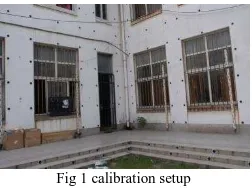
In the following section, a numerical example based on actual experiments will be used to examine the camera model and the parameter estimation strategy described in the previous sections. The setup used in our calibration experiments is shown in Fig. 1.
Fig 1 calibration setup
In this calibration field, 58 mark points are mounted on the walls and steps. These points are measured by the total station, whose angle measurement accuracy and ranging accuracy are 1″ and 0.6mm+2ppm, respectively. To promise the accuracy of every point within the millimeter level, the measuring distance is less than 100 meters, and every point is measured 4 times. The weights for the 3D object coordinates are equal.
These 58 mark points are divided into two groups, including 38 control points and 20 check points.
The images were taken by the consumer-grade camera: Nikon D200, in which the effective part of the CCD sensor array is 3872
2592 pixels (23.6mm×15.8mm) and the focal length is about 50 mm.The corresponding image-point locations are estimated with sub-pixel accuracy.
In the experiment, eight camera stations are set up, and one image is taken on every station. The shooting distance is between 15 and 20 meters. The sample is presented as Fig.2, and the 38 control points are remarked by red crosses.
Fig 2 the sample of images taken by the camera
After the initial values are calculated by formula (2) and (3) with LS adjustment, the improved two-step calibration method is proceeded to optimize all the calibration parameters by formula (9) and (10). In order to solve this adjustment problem, we compute this step by using the WLS and WTLS method, respectively. For the EIV model, we use the solution within the iteratively linearized GH model. The weights for the six pseudo-observation equations are 1010. So the covariance matrix is:
3
The estimated calibration results are displayed in Table 1. The evaluation method is the multi-image intersection described in section 4. The precision and accuracy of the solution will be evaluated by control points and check points respectively. With the formula (34) and (35), the 3D object world coordinates of every point can be solved. Then the difference between the
represent the variance components of the ground control points and check points; 2 evaluation results are shown in Table 2 and Table 3.
Tab.1 Calibration results
Classical two-step method Improved two-step method
LS WLS WTLS
S 1.000269 1.000269 1.000267
1
Tab.2 Precision of the calibration results calculated by control points Classical two-step method Improved two-step method
LS WLS WTLS
Tab.3 Accuracy of the calibration results calculated by check points Classical two-step method Improved two-step method
LS WLS WTLS
Comparing the results for the calibration parameters from Tables 1 and the evaluation results in Tables 2 and Table 3, differences can be analyzed.
1) As can be seen from the calibration results shown in Table 3, the offsets of the principle point and many kinds of parameters for camera distortion cannot be obtained by the classical two-step calibration method. But for this lens, the decentering and thin prism distortions should not be neglected.
2) As shown in Table 1, no matter which calculation procedure is chosen, the calibration results solved by the improved two-step method are similar.
3) From the evaluation results in Table 2, the variance component of the control points solved by improved two-step calibration method is less than 1.5 millimeters, which is smaller than the one calculated by the classical two-step method. And from Table 3, we can see that the accuracy of the calibration results calculated by the improved two-step calibration method is higher than the classical one. However, if the camera calibration model is the same, for example, as the improved two-step calibration method, with the EIV model, we can obtain higher accurate calibration results than with the GM model. 4) Since the errors are obviously distributed in both the object world coordinate system and the image coordinate system, the EIV model is preferable for solving this calibration problem. This can be detected also from the evaluation results in Table 2 and Table 3. The variance components calculated by the EIV model are much smaller than those calculated by the GM model.
6. CONCLUDING REMARKS
This contribution investigates an improved calibration method for consumer-grade cameras. And to adjust this nonlinear improved model, the solution within the EIV model is used to compute the optimal calibration parameters. Then the multi-image intersection is applied to evaluate accuracy of the camera calibration results. Finally, a real example is employed to demonstrate this improved two-step calibration model and process the solution within the iteratively linearized GH model. The conclusions are summarized as follows:
1) Unlike the classical two-step method, which can only handle radial distortion, the improved method proposed here can synthetically establish a camera model that accounts for major sources of camera distortion, namely, radial, decentering, and thin prism distortions. Because the consumer-grade camera usually consists of more distortion than a metric camera, distortion correction is essential here. So the correction of radial and tangential distortion simultaneously can result in a considerable improvement over just correcting radial distortion. 2) Besides the more reasonable distortion correction, the improved method can also calculate the coordinates of principle points at the same time. And the last step is to optimize all of the calibration parameters with the initial value calculated by the classical two-step calibration method. So the reliability and accuracy is improved and the convergence is sped up.
3) Based on the fact that random errors exist both in the object world coordinate system and the image coordinate system, an EIV model is preferable for solving this calibration problem. After evaluation by the multi-image intersection, accuracy results present that variance components of the control points which are calculated by the EIV model are much smaller than those calculated by the GM model. So the accuracy has been improved.
4) During the calculation processing, a covariance matrix in a general form can be employed with different variance for every point and with correlation between coordinates. In other words, the nonlinear calibration model can be solved without any problems, no matter whether the weight matrix is diagonal or not.
On all accounts, the presented improved two-step calibration method can solve the calibration problems more stably and reasonably. To solve this problem, the solution within the iteratively linearized GH model can be used as an alternative WTLS method for computing an exact solution, but is more general with respect to the possible weight matrices.
7. ACKNOWLEDGEMENT
The paper is substantially supported by The National Natural Science Fund Projects of China “Research On The Methodology And Application Of Robust Total Least Squares” (No. 41074017). The author would like to thank Pro. Yi Chen for his substantial help.
REFERENCES
Brown, D. C., 1966. Decentering distortion of lenses. Photometric Eng. Remote Sensing, 32 (3) , pp. 444-462. Faig, W., 1975. Calibration of close-range photogrammetric systems: Mathematical formulation. Photogrammetric Eng. Remote Sensing, 41 (12), pp. 1479-1486.
Faugeras, O. D. and Toscani, G., 1986. Calibration problem for stereo. Proc. Int. Conf Comput. Vision Putt. Recogn. (Miami Beach, FL), pp. 15-20.
Ganapathy, S., 1984. Decomposition of transformation matrices for robot vision. Proc. IEEE Int. Conf Robotics Auromut. (Atlanta), pp. 130-139.
Neitzel, F., 2010. Generalization of total least-squares on example of unweighted and weighted 2D similarity transformation. J Geodesy, 84 (12), pp. 751-762.
Pope, A.J., 1972. Some pitfalls to be avoided in the iterative adjustment of nonlinear problems. Proceedings of the 38th Annual Meeting of the American Society of Photogrammetry, Washington, DC, pp. 449–477.
Schaffrin, B., 2006. A Note on Constrained Total Least-Squares Estimation. Linear Algebra and its Applications, 417, pp. 245-258.
Schaffrin, B. and Felus, Y. A., 2008. On the Multivariate Total Least-Squares approach to empirical coordinate transformation: Three algorithms. J Geodesy, 82 (6), pp. 373-383.
Schaffrin, B., and Wieser, A., 2008. On weighted Total Least-Squares adjustment for linear regression, J Geodesy , 82(7), pp. 415-421.
Schaffrin, B. and Felus, Y. A., 2009. An algorithmic approach to the total least-squares problem with linear and quadratic constraints, Stud. Geophys. Geod., 53, pp. 1-16.
Schaffrin B., Neitzel F. and Uzum S., 2009. Empirical similarity transformation via TLS-adjustment: exact solution vs. Cadzow’s approximation, International Geomatics Forum, Qingdao, People’s Republic of China, pp. 28-30.
Tsai, R. Y., 1987. A versatile camera calibration technique for high-accuracy 3D machine vision metrology using off-the-shelf TV cameras and lenses. IEEE J. Robotics Automat., RA-3 (4), pp. 323-344.
Van Huffel, S. and Vandeualle, J., 1991. The total least squares problem. Computational Aspects and Analysis, Frontiers in Applied, Mathematics, SIAM, Philadelphia: 9, pp. 1-87. Wackrow, R., Chandler, J. H. and Bryan, P., 2007. Geometric consistency and stability of consumer-grade digital cameras for accurate spatial measurement. Photogrammetric Record, 22(118), pp. 121–134.
Wackrow, R. and Chandler, J. H., 2008. A convergent image configuration for DEM extraction that minimizes the systematic effects caused by an inaccurate lens model. Photogrammetric Record, 23(121), pp. 6–18.
Weng, J., Cohen, P., and Herniou, M., 1992. Camera Calibration with Distortion Models and Accuracy Evaluation. IEEE Transactions on Patten Analysis and Machine Intelligence, 14 (10), pp. 965-980.
Wong, K. W., 1975. Mathematical formulation and digital analysis in close-range photogrammetry. Photogrammetric Eng. Remote Sensing, 41 (11), pp. 1355-1373.