Chp06 – Bernoulli & Poisson Process

Introduction to Probability

SECOND EDITION

Dimitri

P.

Bertsekas and John N. Tsitsiklis

Massachusetts Institute of Technology

WWW site for book information and orders

http://www.athenasc.com

6

The Bernoulli and Poisson Processes

6. 1 . The Bernoulli ProcelSs .

6.2. The Poisson Process

6.3. Summary and Discussion

Problems . . .

.

Contents

·

p. 297

·

p. 309

·

p. 324

·

p. 326

296 The Bernoulli and Poisson Processes Chap. 6

A

stochastic process is a mathematical model of a probabilistic experiment that

evolves in

time

and generates a sequence of numerical values. For example. a

stochastic process can be used to model:

(a) the sequence of daily prices of a stock;

(b) the sequence of scores in a foot ball game:

(c) the sequence of failure times of a machine:

(d) the sequence of hourly traffic loads at a node of a communication network;

(e) the sequence of radar mea.'iurements of the position of an airplane.

Each numerical

value

in the sequen('e is modeled by a random variable, so a

stochastic process is simply a (finite or infinite) sequence of random variables

and does not represent a major conceptual departure from our basic framework.

We are still dealing with a single basic experiment that involves outcomes gov­

erned by a probability law. and random variables that inherit their probabilistic

properties from that law.

t

However. stochastic processes involve some change in emphasis over our

earlier models. In particular:

(a)

"Ve

tend to focus on the

dependencies

in the sequence of values generated

by the process. For example. how do future prices of a stock depend on

past values?

(b) We are often interested in

long-term averages

involving the entire se­

quence of generated values. For example. what is the fraction of time that

a machine is idle?

(c) 'Ve sometimes wish to characterize the likelihood or frequency of certain

boundary events.

For example, what is the probability that within a

given hour all circuits of some telephone system become simultaneously

busy: or what is the frequency with which some buffer in a computer net­

work overflows with data?

There is a wide variety of stochastic processes. but in this book we will

only discuss two major ('ategories.

(i)

Arrival-

Type Processes :

_{Here. we are interested in occurrences that have}

the character of an "'arrivaL"' such as message receptions at a receiver, job

completions in a manufacturing celL customer purchases at a store, etc.

We will focus on models in which the interarrival times (the times between

successive arrivals) are independent random variables. In Section

6 . 1 ,

we

consider the case where arrivals occur in discrete time and the interarrival

t Let us empha..<;ize that all of the random variables arising in a stochastic process

Sec. 6. 1 The Bernoulli Process 297

times are geometrically distributed - this is the

Bernoulli process .

_{In Sec­}

tion

6.2,

we consider the case where arrivals occur in continuous time and

the interarrival times are exponentially distributed - this is the

Poisson process .

(ii)

Markov Processes :

_{Here, we are looking at experiments that evolve in time}

and in which the future evolution exhibits a probabilistic dependence on

the past. As an example, the future daily prices of a stock are typically

dependent on past prices. However. in a Markov process� we assume a very

special type of dependence: the next value depends on past values only

through the current value. There is a rich methodology that applies to

such processes, and is the subject of Chapter 7.

6.1 THE BERNOULLI PROCESS

The Bernoulli process can be visualized as a sequence of independent coin tosses,

where the probability of heads in each toss is a fixed number

p

in the range

o

<

p

_<

1 .

In general, the Bernoulli process consists of a sequence of Bernoulli

trials. Each trial produces a

1

(a success) with probability

p,

and a

0

(a failure)

with probability

1

-

p,

independent of what happens in other trials.

Of course, coin tossing is just a paradigm for a broad range of contexts

involving a sequence of independent binary outcomes. For example, a Bernoulli

process is often used to model systems involving arrivals of customers or jobs at

service centers. Here, time is discretized into periods� and a "success" at the kth

trial is associated with the arrival of at least one customer at the service center

during the kth period. We will often use the term "arrival" in place of "success"

when this is justified by the context.

In a more formal description, we define the Bernoulli process as a sequence

Xl � X2 ,

.

. .

of

independent

Bernoulli random variables

Xi

with

for each i.t

P(

Xi

=

1 )

=

P(success at the ith trial)

=

p,

P(

Xi =

0)

=

P(failure at the ith trial)

=

1

-

p,

Given an arrival process, one is often interested in random variables such

as the number of arrivals within a certain time period. or the time until the first

arrival. For the case of a Bernoulli process, some answers are already available

from earlier chapters. Here is a summary of the main facts.

298 T1Je Bernoulli and Poisson Processes Chap. 6

Some Random Variables Associated with the Bernoulli Process and their Properties

• The binomial with parameters

p

and

n.

This is the number S of

successes in

n

independent trials. Its PMF, mean, and variance are

k 0, 1, . ..

, n,

The independence assumption underlying the Bernoulli process has important

implications. including a memorylessness property

(

whatever has happened in

past trials provides no information on the outcomes of future trials

)

. An appre­

ciation and intuitive understanding of such properties is very useful, and allows

the quick solution of many problems that would be difficult with a more formal

approach. In this subsection. we aim at developing the necessary intuition.

Let us start by considering random variables that are defined in terms of

what happened in a certain set of trials. For example. the random variable

Z

= (Xl

+

X3)X6X7

is defined in terms of the first, third. sixth, and seventh

Sec. 6. 1 The Bernoulli Process 299 whereas V is determined by the even-time sequence X2 • X4 , . . .. Since these two sequences have no common elements, U and V are independent.

Suppose now that a Bernoulli process has been running for

n

time steps,

and that we have observed the values of Xl , X2 , . . . , Xn . We notice that the

sequence of future trials Xn+l , Xn+2, . . . are independent Bernoulli trials and

therefore form a Bernoulli process. In addition, these future trials are indepen­

dent from the past ones. We conclude that starting from any given point in

time, the future is also modeled by a Bernoulli process, which is independent of

the past. We refer to this loosely as the

fresh-start

property of the Bernoulli

process.

Let us now recall that the time

T

until the first success is a geometric

random variable. Suppose that we have been watching the process for

n

time

steps and no success has been recorded. What can we say about the number

T-n

of remaining trials until the first success? Since the future of the process

(

after

time

n)

is independent of the past and constitutes a fresh-starting Bernoulli

process, the number of future trials until the first success is described by the

same geometric PMF. Mathematically, we have

P

(

T - n

=

t i T > n)

=

( 1

-

p)t-Ip

=

P

(

T

=

t), t

=

1 , 2, . . . .

We refer to this as the

memorylessness

property. It can also be derived al­

gebraically, using the definition of conditional probabilities, but the argument

given here is certainly more intuitive.

Independence Properties of the Bernoulli Process

•

For any given time

n,

the sequence of random variables X

n+ 1 ,

X

n+2,

.

.

.

(

the future of the process

)

is also a Bernoulli process, and is indepen­

dent from

Xl , . ' " Xn

(

the past of the process

)

.

•

Let

n

be a given time and let

T

be the time of the first success after

time

n.

Then,

T - n

has a geometric distribution with parameter

p,

and is independent of the random variables

X I,

. . . ,Xn.

Example 6.2. A computer executes two types of tasks, priority and non priority, and operates in discrete time units (slots). A priority task arrives with probability

p at the beginning of each slot, independent of other slots, and requires one full slot to complete. A nonpriority task is always available and is executed at a given slot if no priority task is available. In this context, it may be important to know the probabilistic properties of the time intervals available for non priority tasks.

300

(a) =

(b) B =

(c) I ;;

B I

T Z

B

Z

mean,

first busy

up to

6. 1 : I l l ustrat ion of random and and idle in 6 . 2 . In t he top _T = 4, B = 3, I = 2, and Z 3. In t he

bottom _T I , 1 = 5) B = 4, and Z = 4 .

6

Sec. 6. 1 The Bernoulli Process of the first busy slot, so that

PI (k)

=

(1 - p)k-lp,

k =

1, 2, . . .

, var(I) =

I - p

P

301

We finally note that the argument given here also works for the second, third, etc., busy (or idle) period. Thus, the PMFs calculated above apply to the ith busy and idle period, for any i.

If we start watching a Bernoulli process at a certain time

n,

what we see

is indistinguishable from a Bernoulli process that has just started. It turns out

that the same is true if we start watching the process at some

random

time N,

as long as N is determined only by the past history of the process and does

not convey any information on the future. Indeed, such a property was used in

Example 6.2, when we stated that the process starts fresh at time

L + 1 .

For

another example, consider a roulette wheel with each occurrence of red viewed

as a success. The sequence generated starting at some fixed spin (say, the 25th

spin) is probabilistically indistinguishable from the sequence generated starting

immediately after red occurs in five consecutive spins. In either case, the process

starts fresh (although one can certainly find gamblers with alternative theories) .

The next example makes a similar argument, but more formally.

Example 6.3. Fresh-Start at a Random Time. Let

N

be the first time that we have a success immediately following a previous success. (That is,

N

is the first

i for which

Xi-l

=

Xi

=

1 . ) What is the probability

P(XN+l

=

XN+2

=

0)

that there are no successes in the two trials that follow?

6

An IS

of the kth success (or

is the kth interarrival

we

by Tk . de

note

It is

b

y

Yk . A

related random

by

variable

1 ,

k =

number

(k

- 1

)st success until

for an illustration,

and also

note that

+ + .

.

. +

6.2: Illustration of interarrival w here a 1 represents an arrivaL I n

= 2, T4 = 1 . Y1 = 3 , = 8,

We have already seen

with

p. a

success

T1 ,

a new Bernoulli process,

to the original: the

T2

until

next success has the same geometric

PfvlF.

Furthermore, past trials (up to and

including

T1 ) are

(from

1

is determined exclusively by what happens

see that T2 is

of Tl . Continuing

random

distribution.

. . . . are

This important observation

to an

describing the Bernoulli

which is

Alternative

1 .

with

a

sequence

co

m

m

o

n

the

more

way of

Sec. 6. 1 The Bernoulli Process 303

Example 6.4. It has been observed that after a rainy day. the number of days until it rains again is geometrically distributed with parameter p. independent of t he past . Find the probability that it rains on both t he 5th and the 8th day of t he month.

If we attempt to approach t his problem by manipulating the geometric PMFs in the problem statement. t he solution is quite tedious. However, if we view rainy days as "arrivals," we notice that t he description of the weather conforms to the al­ ternative description of the Bernoulli process given above. Therefore, any given day is rainy with probability p. independent of other days. In particular. the probability that days 5 and 8 are rainy is equal to p2 .

The kth Arrival Time

The time

Yk

of the kth success (or arrival) is equal to the sum

Yk

=

Tl

+

T2 +

.

. .

+

Tk

of k independent identically distributed geometric random variables.

This allows us to derive formulas for the mean. variance. and Pl\IF of Yk . which

are given in the table that follows.

Properties of the kth Arrival Time

•

The kth arrival time is equal to the sum of the first

k

interarrival times

and the latter are independent geometric random variables with com­

mon parameter

p.

•

The mean and variance of

Yk

are given by

k(l

p)

var(Yk )

=

var(TI )

+ ... +

var(Tk)

=

2 .

P

•

The PMF of

Yk

is given by

(t -1)

P

_Y

k

(

t

)

=

k

-1

pk (l - p)t-k,

t=k,k+1, ...

,

and is known

as

the

Pascal PMF of order k.

304 The Bernoulli and Poisson Processes Chap. 6

comes at time

t)

will occur if and only if both of the following two events

A

and

B

occur:

(

a

)

event

A:

trial

t

is a success:

(

b

)

event

B:

exactly

k - 1

successes occur in the first

t

-

1

trials.

The probabilities of these two events are

and

P(A)

= p,

(

t

- 1

)

P(B)

= pk- l ( l - p)t-k .

k - 1

respectively. In addition. these two events are independent

(

whether trial

t

is a

success or not is independent of what happened in the first

t

- 1

trials

)

. Therefore,

(

t

-

1

)

PYk (t)

=

P(Yk

=

t)

₌

P(A

n

B)

=

P(A)P(B)

₌

k

_

1

pk ( l - p)t - k .

as

claimed.

Example 6.5. In each minute of basketball play� Alicia commits a single foul with probability p and no foul with probability

1 -

p. The number of fouls in different minutes are assumed to be independent. Alicia will foul out of the game once she commits her sixth foul. and will play

30

minutes if she does not foul out. What is the PMF of Alicia�s playing time?

We model fouls as a Bernoulli process with parameter p. Alicia's playing time Z is equal to Y6 • the time until the sixth foul, except if Y6 is larger than

30,

in which case. her playing time is

30;

that is, Z = min

{

Y6 ,

3D}.

The random variable Y6 has a Pascal PMF of order 6, which is given by

(

t

-

1

)

6 t -6

PY6

(t)

=

₅

P

( 1

-

p)

.

t

= 6, 7, . ..

To determine the PMF

pz (z)

of Z, we first consider the case where z is between 6

and 29. For

z

in this range, we have

z

= 6, 7, . . . , 29.

The probability that Z

=

30

is then determined from

29

pz (30)

₌

1

-

L PZ(z).

6. 1

with a Bernoulli process i n which there is a probability p of an

time� consider it as follows. is an arrival. we

choose to it (with probability q) . or to it

(

with probabili

t

y

1 -q) : see Fig. 6.3. Assume that t he decisions to keep or discard are independent

we

on of

are

we see

that it is a Bernoulli process: in each time slot . there is a probability pq of a

a reverse

(with

parameters p

as

follows.

All

the same reason . process. with a probability

to p( 1 - q) .

6.3: Splitt ing of a Bernoulli process .

. we st�rt h t·wo

q . respectively) and

IS in t he lllcrged if therc

is an at one two

probabilit,\' p + q - pq

[

one minus probability

(1

-

p) ( I

- q) of no arrival in either process]. Since different time slots in

slot� are

the nlerged process is Bernoulli. with success probability p + q - at each t i nle

6.4.

of successes n

with parameters n. and p.

In

work

center Ina,," see a streanl of

to a

be faced

w

ith arrivals :stream .

IS a

6

of Bernoulli processes .

•

k 1 ,

mean are

Sec. 6. 1 The Bernoulli Process 307

•

For any fixed nonnegative integer

k,

the binomial probability

n'

ps(k)

=

(n

_

k!

.

pk(1 - p)n-k

converges to

pz(k),

when we take the limit

as

n

-+ 00

and

p

=

)./n,

while keeping ). constant.

•

In general, the Poisson PMF is a good approximation to the binomial

as

long

as

).

=

np, n

is very large, and

p

is very small.

To verify the validity of the Poisson approximation, we let

p )./n

and

note that

n!

ps(k)

=

_(n

_

_{k)! k! . pk(1 - p)n}

-k

n(n - l) . . .

).k . (

_{1 -}

).)n-k

k!

nk

n

n (n 1) . . . (n - k + l) .

).k . (

_{1 -}

�)n-k

n

n

n

k!

n

Let us focus on a fixed

k

and let

n

-+ 00.

Each one of the ratios

(n - 1)/n,

(n - 2)/n, . . . , (n - k + 1)/n

converges to

1.

Furthermore,t

( ).)-k

_{1 - ;,}

-+

1,

We conclude that for each fixed

k,

and

as

n

-+ 00 ,

we have

).k

ps(k)

-+

eA

-k! .

Example 6.6. As a rule of thumb, the Poisson/binomial approximation

->.

>.k

n!

k(

e

k!

� (n _

k)! k!

.

P

1

P ,

)n-k

k

=

0, 1 , . . . , n,

is valid to several decimal places if n � 100,

P

:$ 0.01, and >' = np. To check this, consider the following.

Gary Kasparov, a world chess champion, plays against 100 amateurs in a large simultaneous exhibition. It has been estimated from past experience that Kasparov

t We are using here, the well known formula limx ... oo ( l -

�

)x

=

e- 1 • Letting

308 The Bernoulli and Poisson Processes Chap. 6 wins in such exhibitions

99%

of his games on the average (in precise probabilistic terms, we assume that he wins each game with probability

0.99,

independent of other games) . What are the probabilities that he will win

100

games,

98

games,

95

games, and

90

games?

We model the number of games

X

that Kasparov does not win as a binomial random variable with parameters n =

100

and

p

=

0.01 .

Thus the probabilities that he will win

100

games,

98, 95

games, and

90

games are

px (0)

=

(1 - 0.01) 100

=

0.366,

100!

2

₉₈

px (2)

=

_{98. 2.}

· 0.01 (1 - 0.01)

=

0.185,

100!

5

₉₅

px (5)

=

_{95! 5! · 0.01 ( 1 - 0.01)}

=

0.00290,

(10)

=

100! . 0 0110(1 - 0 01)90

=

7 006 . 10-8

px

_{90! 1O!}

_'

.

.

_,

respectively. Now let us check the corresponding Poisson approximations with >' =

100 · 0.01

=

1.

They are:

pz (O)

= e - l

�

_O.

=

0.368,

pz (2)

= e - l

�

=

0.184,

2.

pz (5)

=

e- 1

₌

0.00306,

pz (lO)

=

e- 1

�

=

1.001 . 10-8.

10.

By comparing the binomial PMF values

px (k)

with their Poisson approximations

pz (k),

we see that there is close agreement.

Suppose now that Kasparov plays simultaneously against just

5

opponents. who are, however, stronger so that his probability of a win per game is

0.9.

Here are the binomial probabilities

px (k)

for n =

5

and

p

=

0. 1,

and the corresponding Poisson approximations

pz(k)

for >. =

np

=

0.5:

k

0

1

2

3

4

5

px (k)

0.590 0.328 0.0729 0.0081 0.00045 0.00001

pz (k)

0.605 0.303 0.0758 0.0126 0.0016 0.00016

We see that the approximation, while not poor, is considerably less accurate than in the case where n =

100

and

p

=

0.01.

Sec. 6.2 _{The Poisson Process} 309 error, independent of errors in the other symbols. How small should

n

be in order for the probability of incorrect transmission (at least one symbol in error

)

to be less than 0.001?

Each symbol transmission is viewed as an independent Bernoulli trial. Thus,

the probability of a positive number

S

of errors in the packet is

1

- P(S

=

0)

= 1 - ( 1

- p)" .

applies to situations where there is no natural way of dividing time into discrete

periods.

To see the need for a continuous-time version of the Bernoulli process. let

us consider a possible model of traffic accidents within a city. \Ve can start by

discretizing time into one-minute periods and record a " success" during every

minute in which there is at least one traffic accident. Assuming the traffic in­

tensity to be constant over time, the probability of an accident should be the

same during each period. Under the additional (and quite plausible) assumption

that different time periods are independent. the sequence of successes becomes a

Bernoulli process. Note that in real life. two or more accidents during the same

one-minute interval are certainly possible, but the Bernoulli process model does

not keep track of the exact number of accidents. In particular. it does not allow

us to calculate the expected number of accidents within a given period.

One way around this difficulty is to choose the length of a time period to be

very small. so that the probability of two or more accidents becomes negligible.

But how small should it be? A second? A millisecond? Instead of making an

arbitrary choice, it is preferable to consider a limiting situation where the length

of the time period becomes zero. and work with a continuous-time model.

We consider an arrival process that evolves in continuous time. in the sense

that any real number

t

is a possible arrival time. We define

310 The Bernoulli and Poisson Processes Chap. 6

and assume that this probability is the same for all intervals of the same length ,.

We also introduce a positive parameter A, called the

arrival rate

or

intensity

of the process, for reasons that will soon become apparent.

Definition of the Poisson Process

An arrival process is called a Poisson process with rate A if it has the fol­

lowing properties:

(a)

(Time-homogeneity)

The probability

P(k, ,)

of

k

arrivals is the

same for all intervals of the same length ,.

(b)

(Independence)

The number of arrivals during a particular interval

is independent of the history of arrivals outside this interval.

(c)

(Small interval probabilities)

The probabilities

P(k, ,)

satisfy

P(O, ,)

=

1

-

A, +

0

(

,

)

,

P(l, ,)

=

A, + OI ('),

P(k, ,)

=

Ok('),

for

k

=

2, 3, . . .

Here,

0

(

,

)

and

Ok

(

,

)

are functions of , that satisfy

. 0

(

,

)

hm

-- = 0,

7"--+0 , 7"--+0

lim

Ok(')

, = 0.

The first property states that arrivals are " equally likely" at all times. The

arrivals during any time interval of length , are statistically the same, i.e., they

obey the same probability law. This is a counterpart to the assumption that the

success probability

p

in a Bernoulli process is the same for all trials.

To interpret the second property, consider a particular interval

[t, tf],

of

length

tf - t.

The unconditional probability of

k

arrivals during that interval

is

P(k,

tf - t).

Suppose now that we are given complete or partial information

on the arrivals outside this interval. Property (b) states that this information

is irrelevant: the conditional probability of

k

arrivals during

[t, tfl

remains equal

to the unconditional probability

P(k,

tf - t).

This property is analogous to the

independence of trials in a Bernoulli process.

The third property is critical. The

0

(

,

)

and

Ok (

,

)

terms are meant to be

negligible in comparison to " when the interval length , is very small. They can

be thought of as the

0(,2)

terms in a Taylor series expansion of

P(k,

,

)

.

Thus,

for small " the probability of a single arrival is roughly A" plus a negligible

term. Similarly, for small " the probability of zero arrivals is roughly 1

-

A,.

Finally, the probability of two or more arrivals is negligible in comparison to

We

3 1 1

are

has one arrival with probability

to A61 or

z

e

r

o with probability approxi mately

Therefore, the process being studied can be approxinlated by a Bernoulli proce

s

s

1

the approximatioll Inore more as 0 becomes smaller.

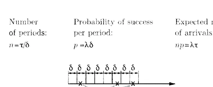
Figure 6 . 5 : _{Bernoulli approximation o f the Poisson process over a n interval o f}

length r .

The probability

P(

k: of k in r is

the ( binomial) probability of _k succetises in n = T / fJ

i

nd

e

pe

nd

ent

with success probability _p

=

_{,\<5 .} While keeping the length T of

interval fixed � we let the to zero. We then note that the

nu_rnbe_{r n of periods goes} to _infinity, whi le the product up rcrnain::s consta

nt

_and

to Ai. t

h

e_se _{we saw} in the previous that

binomial PMF converges to a Po

i

sson _Pi\lF with parame

t

er AT. \Ve are then led to

Note a Taylo

r

_

- AT ( '\ T ) k

P(k�

T

) -

e

_{k"l ' k}

= 0, 1 , . . . .

of e - AT yiel

d

s P(O, T ) = e - AT = 1 - + O(T) �

312 The Bernoulli and Poisson Processes Chap. 6

Using our earlier formulas for the mean and variance of the Poisson PMF.

we obtain

E[NTJ = AT.

var

(

NT

)

= AT.

where

NT

denotes the number of arrivals during a time interval of length

T.

These formulas are hardly surprising. since we are dealing with the limit of a

binomial PMF with parameters

n = Tlb, P = Ab.

mean

np = AT,

and variance

np( 1 - p) � np = AT.

Let us now derive the probability law for the time T of the first arrival,

assuming that the process starts at time zero. ;.rote that we have

T > t

if and

only if there are no arrivals during the interval

[0.

t

J.

Therefore.

FT(t)

= P(

T

< t)

= 1 -P(

T

>

t)

= 1 - P(O,

t)

= 1 - e�M. t > O.

We then differentiate the CDF

FT(t)

of T, and obtain the PDF formula

t > O.

which shows that the time until the first arrival is exponentially distributed with

parameter

A.

We summarize this discussion in the table that follows. See also

Fig. 6.6.

Random Variables Associated with the Poisson Process and their Properties

• The Poisson with parameter AT.

This is the number

N"

of arrivals

in a Poisson process with rate

A,

over an interval of length

T.

Its PMF,

mean, and variance are

A (AT)k PN,, (k) = P(k, T) = e- "

k! ' k = O, l , . . . ,

var

(

NT

)

= AT .

• The exponential with parameter A.

This is the time T until the

first arrival. Its PDF, mean, and variance are

!T(t)

= Ae-At ,

t

2:

0,

v

ar

(

T

)

= 1 A2 '

Example 6.8. You get email according to a Poisson process at a rate of A = 0.2

6 . 6 : _{View of the Bernoulli process as the discrete-time version}

process. We d iscretize time in smal l intervals 6 _{and associate} each interval with a Bernoulli trial whose is p = AO. The table summarizes some of the basic

is preceding

314 The Bernoulli and Poisson Processes Chap. 6 length 15. and has therefore a Poisson distribution with parameter 10 · 15 = 150.

This example makes a point that is valid in general. The probability of

k

process, including the independence of nonoverlapping time sets, and the mem­

orylessness of the interarrival time distribution. Given that the Poisson process

can be viewed

as

a limiting ca..<;e of a Bernoulli process. the fact that it inherits

the qualitative properties of the latter should be hardly surprising.

Independence Properties of the Poisson Process

•

For any given time

t

>

0,

the history of the process after time

t

is also

a Poisson process, and is independent from the history of the process

until time

t.

•

Let

t

be a given time and let

T

be the time of the first arrival after

time

t.

Then,

T

-

t

has an exponential distribution with parameter

�,

and is independent of the history of the process until time

t.

The first property in the above table is establ

�

shed by observing that the

portion of the process that starts at time

t

satisfies the properties required by

the definition of the Poisson process. The independence of the future from the

past is a direct consequence of the independence assumption in the definition

of the Poisson process. Finally, the fact that

T

-

t

has the same exponential

distribution can be verified by noting that

P(T

-

t

>

s

)

=

P

(0

arrivals during

[t, t + s

J

)

= P(O, s

)

=

e->'s.

Sec. 6.2 _{The Poisson Process 315}

Example 6.10. You and your partner go to a tennis court, and have to wait until the players occupying the court finish playing. Assume (somewhat unrealistically) that their playing time has an exponential PDF. Then, the PDF of your waiting time (equivalently, their remaining playing time) also has the same exponential PDF, regardless of when they started playing.

Example 6.11. When you enter the bank, you find that all three tellers are busy serving other customers, and there are no other customers in queue. Assume that the service times for you and for each of the customers being served are independent identically distributed exponential random variables. What is the probability that you will be the last to leave?

The answer is 1/3. To see this, focus at the moment when you start service with one of the tellers. Then, the remaining time of each of the other two customers being served, as well as your own remaining time, have the same PDF. Therefore, you and the other two customers have equal probability 1/3 of being the last to leave.

Interarrival Times

An important random variable associated with a Poisson process that starts at

time 0, is the time of the kth arrival, which we denote by

Yk .

A related random

variable is the kth interarrival time, denoted by

Tk •

It is defined by

k

=

2, 3, . . .

and represents the amount of time between the

(

k - l

)

st and the kth arrival.

Note that

We have already seen that the time

Tl

until the first arrival is an exponen­

tial random variable with parameter A. Starting from the time

Tl

of the first

arrival, the future is a fresh-starting Poisson process.

t

Thus, the time until the

next arrival has the same exponential PDF. Furthermore, the past of the process

(

up to time

T1 )

is independent of the future

(

after time

Tl ) .

Since

T2

is deter­

mined exclusively by what happens in the future, we see that

_T2

is independent

of

T1 •

Continuing similarly, we conclude that the random variables

_{TI , T2, T3,}

.. .

are independent and all have the same exponential distribution.

This important observation leads to an alternative, but equivalent, way of

describing the Poisson process.

316 The Bernoulli and Poisson Processes Chap. 6

Alternative Description of the Poisson Process

1.

Start with a sequence of independent exponential random variables

Tl , T2, . . . , with common parameter A, and let these represent the in­

terarrival times.

2.

Record an arrival at times Tl , Tl

+

_{T2 , Tl}

+

T2

+

T3 . etc.

The kth Arrival Time

The time Y/"o of the kt h arrival is equal to the sum Yk

=

TI

+

T2

+ . . . +

Tk of

k

independent identically distributed exponential random variables. This allows

us to derivE' formulas for t

11('

mean. variance. and PDF of Yk . which are given in

the table that follows.

Properties of the kth Arrival Time

•

The kth arrival time is equal to the sum of the first

k

interarrival times

and the latter are independent exponential random variables with com­

mon parameter A.

•

The mean and variance of Yk are given by

k

var(Yk )

=

var(T1 )

+ . . . +

var(Tk )

=

A2

'

•

The PDF of Yk is given by

y

2: 0,

and is known

(lli

the

Erlang PDF of order k.

To evaluate the PDF

jYk

of Yk . we argue that for a small

b,

the product

Sec. 6.2 The Poisson Process 317

y

and

y

+

<5.t

When

<5

is very small. the probability of more than one arrival

during the interval

[y, y

+

<5]

is negligible. Thus, the kth arrival occurs between

y

and

y

+

<5

if and only if the following two events

A

and

B

occur:

(

a

)

event

A:

there is an arrival during the interval

[y, y

+

<5];

(

b

)

event

B:

there are exactly k

-

1 arrivals before time

y.

The probabilities of these two events are

P(A)

�

A

<5

,

and

P(B)

=

P

(

k

-

1

. y

)

=

Ak- 1 yk-Ie->..y

(

k

_{- I)!} .

Since

A

and

B

are independent, we have

Ak-1yk-le->..y

<5fYk

(y)

�

P(y ::s

Yk

::s

y

+

<5)

�

P(A

n

B)

=

P(A) P(B)

�

A

<5

(k

_

1 )! '

from which we obtain

y ? O.

Example 6.12. You call the IRS hotline and you are told that you are the 56th person in line, excluding the person currently being served. Callers depart according

to

a Poisson process with a rate of

). =

2 per minute. How long will you have to wait on the average until your service starts, and what is the probability you will have to wait for more than 30 minutes?

By the memorylessness property, the remaining service time of the person currently being served is exponentially distributed with parameter 2. The service times of the 55 persons ahead of you are also exponential with the same parameter,

t For an alternative derivation that does not rely on approximation arguments, note that for a given

y

? 0, the event

{Yk

::s

y}

is the same as the event

{

number of arrivals in the interval [0,

y]

is at least

k}.

Thus, the CDF of

Yk

is given by

x

k-l

k-l (). )n

FYk (y)

=

P(Yk

�

y)

=

L P(n. y)

= 1 -

L P(n. y)

= 1 -

L y

n.

.

n=k

n=O

n=O

318 The Bernoulli and Poisson Processes Chap. 6

Computing this probability is quite tedious. On the other hand, since Y is the sum of a large number of independent identically distributed random variables, we can use an approximation based on the central limit theorem and the normal tables.

Splitting and Merging of Poisson Processes

Similar to the case of a Bernoulli process, we can start with a Poisson process

with rate

A

and split it. as follows: each arrival is kept with probability

p

and

discarded with probability

1

-

p,

independent of what happens to other arrivals.

In the Bernoulli case, we saw that the result of the splitting was also a Bernoulli

process. In the present context, the result of the splitting turns out to be a

Poisson process with rate

Ap.

Alternatively, we can start with two independent Poisson processes, with

rates

Al

and

A2,

and merge them by recording an arrival whenever an arrival

occurs in either process. It turns out that the merged process is also Poisson

with rate

Al

+

A2.

Furthermore, any particular arrival of the merged process has

probability

At/(AI

+

A2)

of originating from the first process, and probability

A2/(Al

+

A2)

of originating from the second, independent of all other arrivals

and their origins.

We discuss these properties in the context of some examples, and at the

same time provide the arguments that establish their validity.

Example 6. 13. Splitting of Poisson Processes. A packet that arrives at a node of a data network is either a local packet that is destined for that node (this happens with probability p), or else it is a transit packet that must be relayed to another node (this happens with probability 1 -p) . Packets arrive according to a

Poisson process with rate A, and each one is a local or transit packet independent of other packets and of the arrival times. As stated above, the process of local packet arrivals is Poisson with rate Ap. Let us see why.

\Ve verify that the process of local packet arrivals satisfies the defining prop­ erties of a Poisson process. Since A and p are constant (do not change with time) ,

Sec. 6.2 The Poisson Process 319 We conclude that local packet arrivals form a Poisson process and, in particular. the number of such arrivals during an interval of length T has a Poisson P1,fF with parameter P>'T. By a symmetrical argument, the process of transit packet arrivals is also Poisson, with rate >.(1 -

p).

A somewhat surprising fact in this context is that the two Poisson processes obtained by splitting an original Poisson process are independent: see the end-of-chapter problems.

Example 6. 14. Merging of Poisson Processes. People with letters to mail arrive at the post office according to a Poisson process with rate >' 1 , while people with packages to mail arrive according to an independent Poisson process with rate

>'2 . As stated earlier the merged process, which includes arrivals of both types, is Poisson with rate >'1 + >'2 . Let us see why.

First, it should be clear that the merged process satisfies the time-homogeneity property. Furthermore. since different intervals in each of the two arrival processes are independent, the same property holds for the merged process. Let us now focus on a small interval of length 8. Ignoring terms that are negligible compared to 8,

we have

P(O arrivals in the merged process) � ( 1 - >' 1 8) ( 1 - >'28) � 1 - (>'1 + >'2 )8,

P ( 1 arrival in the merged process) � >'1 8( 1 - >'28) + ( 1 - >'1 8)>'28 � (>'1 + >'2 )8,

and the third property has been verified.

Given that an arrival has just been recorded, what is the probability that it is an arrival of a person with a letter to mail? We focus again on a small interval of length 8 around the current time, and we seek the probability

P( 1 arrival of person with a letter 1 1 arrival).

Using the definition of conditional probabilities, and ignoring the negligible proba­ bility of more than one arrival, this is

P arrival of with a >' 1 8

Generalizing this calculation, we let Lk be the event that the kth arrival corresponds to an arrival of a person with a letter to mail, and we have

Furthermore, since distinct arrivals happen at different times, and since, for Poisson processes, events at different times are independent, it follows that the random variables L1 , L2 , . . . are independent.

Example 6.15. Competing Exponentials. Two light bulbs have independent and exponentially distributed lifetimes Ta and n, with parameters >'a and >'b , respectively. What is the distribution of Z = min{Ta , n } , the first time when a

320 The Bernoulli and Poisson Processes

This is recognized as the exponential CDF with parameter ).a

+

).b. Thus, the mini­ mum of two independent exponentials with parameters ).a and ).b is an exponential with parameter ).a + ).b.

For a more intuitive explanation of this fact, let us think of Ta and Tb as the times of the first arrivals in two independent Poisson processes with rates ).a and ).b, respectively. If we merge these two processes, the first arrival time will be min{Ta , Tb}. But we already know that the merged process is Poisson with rate ).a + ).b, and it follows that the first arrival time, min{Ta , Tb}, is exponential with

parameter ).a

+

).b.

The preceding discussion can be generalized to the case of more than two

processes. Thus, the total arrival process obtained by merging the arrivals of

n

independent Poisson processes with arrival rates AI , . . . , An is Poisson with

arrival rate equal to the sum Al

+ . . . +

An .

Example 6. 16. More on Competing Exponentials. Three light bulbs have independent exponentially distributed lifetimes with a common parameter ).. What is the expected value of the time until the last bulb burns out?

We think of the times when each bulb burns out as the first arrival times in independent Poisson processes. In the beginning, we have three bulbs, and the merged process has rate 3),. Thus, the time Tl of the first burnout is exponential with parameter 3)" and mean 1 /3),. Once a bulb burns out, and because of the memorylessness property of the exponential distribution, the remaining lifetimes of the other two light bulbs are again independent exponential random variables with parameter ).. We thus have two Poisson processes running in parallel, and the remaining time T2 until the first arrival in one of these two processes is now exponential with parameter 2), and mean 1 /2),. Finally, once a second bulb burns out, we are left with a single one. Using memorylessness once more, the remaining time T3 until the last bulb burns out is exponential with parameter ). and mean

1 /),. Thus, the expected value of the total time is

1 1 1

E

[

TI + T2 + T3]

=

3),

+

2),

+

�.

Note that the random variables T1 , T2 , T3 are independent, because of memoryless­ ness. This allows us to also compute the variance of the total time:

1 1 1

var(Tl

+

T2

+

T3) = var(TI )

+

var(T2 )

+

var(T3 ) =

Sec. 6.2 _{The Poisson Process 321}

Bernoulli and Poisson Processes, and Sums of Random Variables

The insights obtained from splitting and merging of Bernoulli and Poisson pro­

cesses can be used to provide simple explanations of some interesting properties

involving sums of a random number of independent random variables. Alter­

native proofs, based for example on manipulating PMFsjPDFs, solving derived

distribution problems, or using transforms. tend to be unintuitive. We collect

these properties in the following table.

Properties of Sums of a Random Number of Random Variables

322 The Bernoulli and Poisson Processes Chap. 6

many component processes, each of which characterizes the phone calls placed by

individual residents. The component processes need not be Poisson: some people

for example tend to make calls in batches� and (usually) while in the process of

talking, cannot initiate or receive a second call. However, the total telephone

traffic is well-modeled by a Poisson process. For the same reasons, the process

of auto accidents in a city� customer arrivals at a store, particle emissions from

radioactive material, etc., tend to have the character of the Poisson process.

The Random Incidence Paradox

The arrivals of a Poisson process partition the time axis into a sequence of

interarrival intervals; each interarrival interval starts with an arrival and ends at

the time of the next arrival. We have seen that the lengths of these interarrival

intervals are independent exponential random variables with parameter A, where

A is the rate of the process. More precisely, for every k, the length of the kth

interarrival interval has this exponential distribution. In this subsection, we look

at these interarrival intervals from a different perspective.

Let us fix a time instant

t*

and consider the length

L

of the interarrival

interval that contains

t* .

For a concrete context, think of a person who shows

up at the bus station at some arbitrary time

t*

and records the time from the

previous bus arrival until the next bus arrival. The arrival of this person is often

referred to as a "random incidence," but the reader should be aware that the

term is misleading:

t*

is just a particular time instance, not a random variable.

We assume that

t*

is much larger than the starting time of the Poisson

process so that we can be fairly certain that there has been an arrival prior to

time

t* .

To avoid the issue of how large

t*

should be, we assume that the Poisson

process has been running forever, so that we can be certain that there has been

a prior arrival, and that

L

is well-defined. One might superficially argue that

L

is the length of a "typicar interarrival interval, and is exponentially distributed,

but this turns out to be false. Instead , we will establish that

L

has an Erlang

PDF of order two.

this is to realize that if we run a

a no nl0ves

Or backward. A nlore formal argument is obtained by noting that

P(t*

- > x

)

=

random

] )

=

P(O, x)

= e - AX ,

with mean 2/ A .

6 . 7 : Illustration o f the random incidence p henomenon. For a fixed time instant f"' , the corresponding i nterarri val i nterval [V, Vj consists of the elapsed

time t* - V and the remain i ng t ime V - t * . These two times are independent

are exponentiaHy dist ributed with A, 50 the PDF of their sum is of order two.

source

probabilistic model i ng.

is that an

at

an

arbitrary time more likely

to

fall

a large than a smal l i nterarrival As a consequence the expected

seen by 1S with 1 / A nlean

exponential A similar situation arises in example that fol lows.

A person shows up at the bus station at a "random!! to mean a

a a person into an

probabi l ity

1/12,

and an interarrival interval of ]ength

5 ·

1

12

+ 55 · = 50. 83 ,

which i s considerably 30,

is

324 The Bernoulli and Poisson Processes Chap. 6

As the preceding example indicates. random incidence is a subtle phe­

nomenon that introduces a bias in favor of larger interarrival intervals, and can

manifest itself in contexts other than the Poisson process. In general, whenever

different calculations give contradictory results, the reason is that they refer to

different probabilistic mechanisms. For instance. considering a fixed

nonran­

dom

k and the associated random value of the kth interarrival interval is a

different experiment from fixing a time

t

and considering the

random

K such

that the Kth interarrival interval contains

t.

For a last example with the same flavor, consider a survey of the utilization

of town buses. One approach is to select a few buses at random and calculate

the average number of riders in the selected buses. An alternative approach is to

select a few bus riders at random, look at the buses that they rode and calculate

the average number of riders in the latter set of buses. The estimates produced

by the two methods have very different statistics, with the second method being

biased upwards. The reason is that with the second method, it is much more

likely to select a bus with a large number of riders than a bus that is near-empty.

6.3

SUMMARY AND DISCUSSION

In this chapter. we introduced and analyzed two memoryless arrival processes.

The Bernoulli process evolves in discrete time, and during each discrete time

step. there is a constant probability

p

of an arrival. The Poisson process evolves

in continuous time, and during each small interval of length

6

>

0, there is a

probability of an arrival approximately equal to

A8.

In both cases, the numbers of

arrivals in disjoint time intervals are assumed independent. The Poisson process

can be viewed as a limiting case of the Bernoulli process, in which the duration

of each discrete time slot is taken to be a very small number

6.

This fact can be

used to draw parallels between the major properties of the two processes, and

to transfer insights gained from one process to the other.

Using the memorylessness property of the Bernoulli and Poisson processes,

we derived the following.

Sec. 6.3 _{Summary and Discussion 325}

326 The Bernou11i and Poisson Processes Chap. 6

P R O B L E M S

SECTION 7.1. The Bernoulli Process

Problem 1 . Each of n packages is loaded independently onto either a red truck (with probability p) or onto a green truck (with probability 1 -p) . Let R be the total number

of items selected for the red truck and let G be the total number of items selected for the green truck.

(a) Determine the PMF, expected value, and variance of the random variable R.

(b) Evaluate the probability that the first item to be loaded ends up being the only one on its truck.

(c) Evaluate the probability that at least one truck ends up with a total of exactly one package.

(d) Evaluate the expected value and the variance of the difference R - G.

(e) Assume that n :2: 2. Given that both of the first two packages to be loaded go onto the red truck, find the conditional expectation, variance, and PMF of the random variable R.

Problem 2. Dave fails quizzes with probability 1/4, independent of other quizzes. (a) What is the probability that Dave fails exactly two of the next six quizzes? (b) What is the expected number of quizzes that Dave will pass before he has failed

three times?

(c) What is the probability that the second and third time Dave fails a quiz will occur when he takes his eighth and ninth quizzes, respectively?

(d) What is the probability that Dave fails two quizzes in a row before he passes two quizzes in a row?

Problem 3. A computer system carries out tasks submitted by two users. Time is divided into slots. A slot can be idle, with probability

PI

= 1/6, and busy with probability

_PB

= 5/6. During a busy slot, there is probability

_PIIB

= 2/5 (respectively,

P21B

= 3/5) that a task from user 1 (respectively, 2) is executed. We assume that events related to different slots are independent.

(a) Find the probability that a task from user 1 is executed for the first time during the 4th slot.

(b) Given that exactly 5 out of the first 10 slots were idle, find the probability that the 6th idle slot is slot 12.

Problems 327

(

d

)

Find the expected number of busy slots up to and including the 5th task from user 1 .

(

e

₎

Find the PMF, mean, and variance of the number of tasks from user 2 until the time of the 5th task from user 1 .

Problem 4 . * Consider a Bernoulli process with probability of success i n each trial equal to p.

(

a

₎

Relate the number of failures before the rth success

(

sometimes called a negative binomial random variable

₎

to a Pascal random variable and derive its PMF.

(

b

₎

Find the expected value and variance of the number of failures before the rth success.

(

c

₎

Obtain an expression for the probability that the ith failure occurs before the rth success.

Solution.

(

a

₎

Let Y be the number of trials until the rth success, which is a Pascal random variable of order r. Let X be the number of failures before the rth success, so that X = Y - r. Therefore, px (k) = py (k + r

)

, and

k

=

0, 1 , . . . .

(

b

)

Using the notation of part

(

a

)

, we have

Furthermore.

E

[

X

]

=

E

[

Y

]

- r

=

� _ r

=

( 1 -p)r.

p p

( 1 -p)r

var

₍

X

₎

=

var

₍

Y

₎

= ₂ .

P

(

c

₎

Let again X be the number of failures before the rth success. The ith failure occurs before the rth success if and only if X 2:: i. Therefore, the desired probability is equal to

i = 1 , 2, . . ..

An alternative formula is derived as follows. Consider the first r +

i - I

trials. The number of failures in these trials is at least i if and only if the number of successes is less than r. But this is equivalent to the ith failure occurring before the rth success. Hence. the desired probability is the probability that the number of successes in r + i - l trials is less than r. which is

i = 1 , 2, . . ..

328 The Bernoulli and Poisson Processes Chap. 6 game with probability

p.

independent of the outcomes of other games. At midnight, you enter his room and witness his losing the current game. What is the PMF of the number of lost games between his most recent win and his first future win?

Solution. Let

t

be the numher of the game when you enter the room. Let !vI be the numher of the most recent pa..c;t game that he won, and let N be the number of the first game to be won in the future. The random variable X

=

N

- t

is geometrically dis­ tributed with parameter

p.

By symmetry and independence of the games, the random variahle Y =

t

-

M

is also geometrically distributed with parameter

p.

The games he

lost hetween his most recent win and his first future win are all the games between

M

and N. Their number L is given by

Problem 6. * Sum of a geometric number of independent geometric random variables. Let Y = Xl + . . . + XN . where the random variables X, are geometric with

parameter

p.

and N is geometric with parameter

q.

Assume that the random variables

N, _{Xl . X2} ... . are independent. Show. without using transforms, that Y is geometric

with parameter

_{pq. Hint:}

Interpret the various random variables in terms of a split Bernoulli process.

Solution. We derived this result in Chapter 4. using transforms. but we develop a more intuitive derivation here. We interpret the random variables _Xi and N as follows. We view the times _{Xl . Xl} + X2 , etc. as the arrival times in a Bernoulli process with parameter

p.

Each arrival is rejected with probability

1 - q

and is accepted with probability q. \Ve interpret N as the number of arrivals until the first acceptance. The process of accepted arrivals is obtained by splitting a Bernoulli process and is therefore itself Bernoulli with parameter pq. The random variable Y = _Xl + . . . + X N is the

time of the first accepted arrival and is therefore geometric. with parameter

pq.

Problem 7. * The bits in a uniform random variable form a Bernoulli pro­ cess. Let Xl , X

2

• • • • be a sequence of binary random variables taking values in the set

{O, I}.

Let Y be a continuous random variable that takes values in the set _[0,

1].

We relate _X and Y by assuming that Y is the real number whose binary representation is 0.X1 X2X3

.

... More concretely. we have

(a) Suppose that the Xi form a Bernoulli process with parameter

p

=

1 /2.

Show that Y is uniformly distributed.

Hint:

Consider the probability of the event

Problems 329 (b) Suppose that

Y

is uniformly distributed. Show that the

Xi

form a Bernoulli

process with parameter p

=

1/2.

Solution. (a) We have

Furthermore,

1

P (Y

E

[0, 1/2])

=

P(XI

=

0)

= 2 =

P (Y

E

_{[1/2, 1] ) .}

1

p(y

E

_{[0, 1/4])}

=

P(XI

= O.

_X2

=

0)

= 4 '

Arguing similarly, we consider an interval of the form

[(

i - I)

/2k

. i

/2k] ,

where i and k

are positive integers and i �

2k .

For

Y

to fall in the interior of this interval, we need

Xl ,

. . . , Xk to take on a particular sequence of values (namely, the digits in the binary

expansion of i - I ) . Hence,

Note also that for any

y

E

[0. 1] '

we have

P(Y

=

y)

=

0,

because the event

{Y

=

y}

can only occur if infinitely many

_XiS

take on particular values, a zero probability event. Therefore, the CDF of

Y

is continuous and satisfies

Since every number

y

in

_{[0, 1]}

can be closely approximated by a number of the form

i/2k.

we have

_P(Y

�

y)

=

y.

for every

y

E

[0, 1] ,

which establishes that

_Y

is uniform. (b) As in part (a). we observe that every possible zero-one pattern for

X I , . . . , X

_k

is associated to one particular interval of the form

[

(i

- 1) /2k

, i

/2k]

for

Y.

These

intervals have equal length, and therefore have the same probability

_{1/2k ,}

since

Y

is uniform. This particular joint PMF for

X

I , . . . •

X

k ,

corresponds to independent

Bernoulli random variables with parameter p =

1/2.

SECTION 7.2. The Poisson Process

Problem

8. During rush hour. from 8 a.m. to 9 a.m., traffic accidents occur according to a Poisson process with a rate of 5 accidents per hour. Between 9 a.m. and

_{1 1}

a.m., they occur as an independent Poisson process with a rate of 3 accidents per hour. What is the PMF of the total number of accidents between 8 a.m. and

_{1 1}

a.m.?

Problem

9. An athletic facility has 5 tennis courts. Pairs of players arrive at the courts and use a court for an exponentially distributed time with mean

40

minutes. Suppose a pair of players arrives and finds all courts busy and k other pairs waiting in queue. What is the expected waiting time to get a court?

Problem

10. A fisherman catches fish according to a Poisson process with rate

330 The Bernoulli and Poisson Processes Chap. 6

(

a

)

Find the probability that he stays for more than two hours.

(

b

)

Find the probability that the total time he spends fishing is between two and five hours.

(

c

)

Find the probability that he catches at least two fish.

(

d

)

Find the expected number of fish that he catches.

(

e

)

Find the expected total fishing time, given that he has been fishing for four hours. Problem 1 1 . Customers depart from a bookstore according to a Poisson process with rate A per hour. Each customer buys a book with probability p, independent of everything else.

(

a

)

Find the distribution of the time until the first sale of a book.

(

b

)

Find the probability that no books are sold during a particular hour.

(

c

)

Find the expected number of customers who buy a book during a particular hour. Problem 12. A pizza parlor serves n different types of pizza, and is visited by a number K of customers in a given period of time, where K is a Poisson random variable with mean A. Each customer orders a single pizza, with all types of pizza being equally likely, independent of the number of other customers and the types of pizza they order. Find the expected number of different types of pizzas ordered.

Problem 13. Transmitters A and B independently send messages to a single receiver in a Poisson manner, with rates of AA and A B , respectively. All messages are so brief that we may assume that they occupy single points in time. The number of words in a message, regardless of the source that is transmitting it, is a random variable with PMF

(

d

)

What is the probability that exactly eight of the next twelve messages received will be from transmitter A?

Problem 14. Beginning at time t = O. we start using bulbs. one at a time, to