Basic Concepts of Primal-Dual in Linear Programming

Basic Concepts of Primal-Dual in Linear Programming

This tutorial is written in order to understand basically what is primal and dual concept in Linear Programming. Understanding this concept will greatly help us in understanding a more advanced op-timization concept such as interior point method algorithm. Before we

1 A Simple Example

Consider the following situation.

Let say that there is two kinds of food (Food A and Food B) made from fish and flour. A portion of Food A need 1 kg fish and

1 kg flour. A portion of Food B need 1/2 kg fish and 1 kg flour. One portion of foodA if sold will gives benefit of 50 cents, while one portion of food B if sold will gives benefit of 30 cents.

If there are 10 kg of fish and 12 kg of flour.

How many portion of food A and B should be made in order to maximize benefit?

Ans

Well, as we see this is a commonLinear Programming(LP) prob-lem. This technique has been normally given in Senior High School Math.

Now let us back on our problem. Let us say that we produce x1 number of portion of food A, and x2 number of portion of food B.

This total production should be constrained by the amount of fish and flour available.

1·x1 + 0.5·x2 ≤ 10 (1) and constraint for the flour is

1·x₁ + 1·x₂ ≤ _{12 (2)}

Objective function is

Z = 50 ·x1 + 30·x2 (3)

If we only produce 1 portion of food A and 1 portion of food B, then the benefit we get will be 50·1 + 30·1 = 80. And we only use 1+0.5

= 1.5kg fish, and 1+1 =2kg flour.

Of course, since producing food A gives more benefit, it is logical to produce more food A than food B.

But we hold that for the moment. Now let solve this LP using sim-plex algorithm.

First we introduce slack variables s1 and s2 into our constraints : So

x₁ + 0.5·x₂ ≤ _{10 (4)}

becomes

x1 + 0.5·x2 +s1 = 10 (5) And

x1 + x2 ≤12 (6)

changes to

x1 +x2 +s2 = 12 (7)

And rewrite the objective function as

Collecting 5, 7 and 8 we obtain the complete equation for simplex algorithm:

x1 + 0.5x2 +s1 = 10 (9)

x₁ +x₂ +s₂ = 12 (10)

Z −50·x1 −30·x2 = 0 (11) Now creating the simplex table:

Table #1

x1 x2 s1 s2 RHS

1 0.5 1 0 10

1 1 0 1 12

Z -50 -30 0 0 0

RHS is right hand size terms.

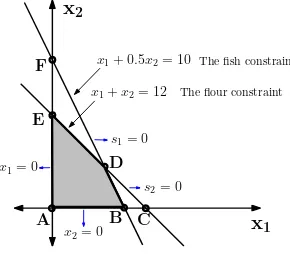
Before we start with simplex algorithm, it is worth to observe the plot of constraints as depicted in Fig. 1.

x

1

Figure 1: The plot of contraints

The area are bounded with lines x1 = 0, x2 = 0, x1 + x2 = 12, 0.5x1 + x2 = 10.

It is interesting to note that the line x₁ + 0.5x₂ = 12 is also called lines₁ = 0, since the constraint with slack variable isx₁+x₂+s₁ = 12, then x₁ +x₂ = 12 is achieved when s₁ = 0.

With similar reasoning, It is interesting to note that the line x₁ +

x2 = 12 is also called line s1 = 0, since the constraint with slack variable is x1 + x2 + s1 = 12, then x1 + x2 = 12 is achieved when

s1 = 0.

The solution of LP programming normally lies on either A or B or D or E points, i.e. at vertex of feasible area OR at line segments of AB or BD or DE or EA. So either on VERTEX or on LINE SEGMENTS. The Simplex Algorithm works by exploiting this fact. It start at A, and then determine whether to go to B or to E, and so on (checking each points at vertex of the feasible area).

Using this fact, let us now start with Simplex Algorithm.

We start from point A ((x1, x2) = (0,0)). Next, where should we go? A or E?

Before we answer this, we observe that there are 6 columns in this simplex table. Second column is x₁ column, and third column is x₂

column.

In Simplex Algorithm, first we should determine, which variable is critical, x1 or x2. Since producing x1 gives benefit 50 (indicated by -50 in x1 column), and x2 which only give benefit 30 (as indicated by -30 in x2 column), therefore we select x1 column, and this correspond to the action that we will go into x1 direction. In other word, we will go to either B or C.

= 600.

It seem that we should go to point C. But from Fig. 1, we observe that point C is not in feasible region. We can only go to point B. So how we know this in simplex?

Using x₁ column as reference, we know that we can use the first row to find B, which is 10/1 = 10 (that is : RHS divide by coef of x₁), and second row to find C which is (12/1=12). We collect this information as a new column (INDIK column). We know that we should choose the smallest value. Selecting x1 column, and first row, we obtain a pivot element which is coloured blue in the following table.

Table #2.

x1 x2 s1 s2 RHS INDIK

1 0.5 1 0 10 10

1 1 0 1 12 12

Z -50 -30 0 0 0

Now we perform elementary row operation using pivot element to eliminate 1 in second row and -50 on the third row, so that in x₁ col-umn, only pivot element is not zero.

second row = second row - first row and

third row = third row + 50 x first row

We obtain (INDIK column is removed again)

Table #3

x₁ x₂ s₁ s₂ RHS

1 0.5 1 0 10

0 0.5 -1 1 2

Z 0 -5 50 0 500

Since column x1 has been chosen, the only x variable left is x2, therefore we choose this column. Since the first row has been chosen, then there is no more choice left except the second row. The element at x2 column on the second row is 0.5. So this is our next pivot (we

Normalize this pivot element to 1 by multiplying second row with 2, we obtain

Again we have to nullize other elements in this column to zero using this pivot element, therefore we perform the elementary row operation

first row = first row - 0.5 x second row

Our optimal solution (x1, x2) = (10,4). And our optimal benefit is 520.

2 Interpretation of Final Simplex Table : Sensitivity of LP

Table #6 shows the final Simplex Table.

x₁ x₂ s₁ s₂ RHS

1 0 2 -1 8

0 1 -2 2 4

Z 0 0 40 10 520

Interesting to observe the score 40 and 10 in the last row. 40 cor-responds to s1 column and s2 corresponds to s2 column.

Oke, our situation is in this problem is, we are limited by the total amount of fish to be 10 unit, and amount of flour are limited by the total amount of 12 unit.

What happen if the amount of fish is increased to 11 and amount of flour is kept constant at 12kg. Will our benefit increase by making more food A or B? How much?

To answer this problem, we again solve it using simplex. Our initial table would be

And our final table is

Table #6B

x1 x2 s1 s2 RHS

1 0 2 -1 10

0 1 -2 2 2

Z 0 0 40 10 560

by 2.

Finally, let us consider the last scenario, we keep the amount of fish to 10 and increase flour from 12 to 13. What is the profit?

Again we solve this problem using simplex.

Initial Table :

In this final table, we see that the total profit is 530, only increase 10 from 520 in initial problem. Now we get better understanding of original final Table. Put it again here :

Table 6

x1 x2 s1 s2 RHS

1 0 2 -1 8

0 1 -2 2 4

Z 0 0 40 10 520

Column s₁ from top to bottom: 2, -2, 40.

This clearly mean that if we add 1 unit of fish, in order to get new optimum, then the production of A should be increased by 2 and production of B should be decreased 2, and the profit is increased by 40.

Column s₂ from top to bottom: -1, 2, 10.

optimum, then the production of A should be decreased by 1 and production of B should be increased by 2, and by doing this, the profit is increased by 10.

This situation has been verified by our examples.

3 Primal-Dual in Linear Programming

In our previous example, we see how simplex method work. Initially we start at Table #1, and finally we arrived at Table #6.

Here we put again Table #1 and Table #6

Table #1

x₁ x₂ s₁ s₂ RHS

1 0.5 1 0 10

1 1 0 1 12

Z -50 -30 0 0 0

Table #6

x1 x2 s1 s2 RHS

1 0 2 -1 8

0 1 -2 2 4

Z 0 0 40 10 520

Now we are talking about the dual form the previous LP problem. The original LP is

Constraints :

x1 + 0.5·x2 ≤ 10 (12)

x1 + x2 ≤12 (13)

Objective function is

The dual of this LP is (change objective to constraint and constraint to objective)

Constraints :

y₁ + y₂ ≥ _{50 (15)}

0.5·y₁ +y₂ ≥ _{30 (16)}

Objective function is to minimize

Y = 10·y1 + 12·y2 (17)

This new LP is called dual of previous LP. Since this one is called

Dual, therefore it makes sense that the original one is called Primal. Observe that

1. objective of primal becomes constraints of dual

2. constraints of primal becomes objective of dual

3. if primal is to maximize then dual is to minimize

4. if primal has constraint of ≤, then dual has constraint of ≥

Introducing new variable r₁ and r₂, the modified LP becomes Con-straints :

y₁ +y₂ +r₁ = 50 (18)

0.5·y1 +y2 + r2 = 30 (19)

Objective function is to minimize

Y = 10·y1 + 12·y2 (20) The plot of constraints is as shown in Fig. 2

y

1

y

₂

A

′

B

′

_C

′

D

′

E

′

F

′ 0.5y₁ + y₂ = 10

r₁ + r₂ = 50

y₁ = 0

y₂ = 0

r₁ = 0

r₂ = 0

Figure 2: The constraints of dual

Table #1C

x₁ x₂ s₁ s₂ RHS

1 0 2 -1 8

0 1 -2 2 4

Z 0 0 40 10 520

Since we are minimizing, please be careful selecting each point, we have to make sure that we are at point A’ then go to either F’, or C’ and so on in feasible region.

Doing this, we arrive in final table as (say that this is as Table #6C).

Table #6C

y₁ y₂ r₁ r₂ RHS

0 1 1 -2 10

1 0 -2 2 40

Y 0 0 -8 -4 520

Table #6

x₁ x₂ s₁ s₂ RHS

1 0 2 -1 8

0 1 -2 2 4

Z 0 0 40 10 520

We see that these two table is very similar. It has the same similar optimal value which is 520. The position of main variable and slack variable in primal and dual are interchanged.

In other word, if we find the optimal value in main variable of the primal, than we know that this is the optimal value for the dual in slack variable, and vice versa.

Even though that physical interpretation of dual in LP is not really obvious, but some at least some aspect has been understood so far.

4 Citation of this work

If you find this work useful, please cite it as follows: