Sci.Int.(Lahore),30(4),523-527 ,2018 ISSN 1013-5316;CODEN: SINTE 8
July-August
ESTIMATING THE PROPORTION IN SMALL AREA
Widiarti1, Shela Malinda T1 , Suharsono S1, Warsono1, and Mustofa Usman1*1
Department of Mathematics, Faculty of Mathematics and Natural Science, Universitas of Lampung, Indonasia Email: [email protected]
ABSTRACT: Small Area Estimation is an indirect prediction used to analyze small areas by utilizing information from larger areas. One of the methods that can be used to estimate in a small area is Hierarchical Bayes (HB). The HB method is usually used for discrete data with multilevel information. Pre-prosperous families are a type of the discrete data that can be classified into two categorical variables by using cluster analysis. In this study, the proportion of pre-prosperous families was suspected to use direct and indirect estimator methods. Analytical calculation is not possible to do on the indirect estimation due to the multidimensional integral form. The numerical calculation was done by Markov Chain Monte Carlo (MCMC) method by using R studio 1.0.143 software. The results of this study showed that the estimated value which was generated by using the indirect estimation had a smaller value when it was compared with the predicted value by using direct estimator. It meant that the indirect estimation was better to estimate the value of the proportion of the pre-prosperous family data.
Keywords: Cluster Analysis, Hierarchical Bayes, Pre-prosperous Family, Markov Chain Montecarlo.
I. INTRODUCTION
Survey is one of the methods used by communities to obtain information from certain areas and becomes one of the important data collecting processes. Survey is conducted to collect information for small areas, for example districts. However, there are some obstacles in collecting information e.g., the unwillingness of respondents to fill questionnaires, the lack of participation of the respondents, and the others. The results of the survey are used to estimate small areas.
Small area estimation is the statistical technique to estimate the parameters of small sample size subpopulations. This estimation technique utilizes data from large areas to predict the concerning variables for smaller areas. The Small area is defined as a small sample size subpopulations so that the direct predictions cannot produce rigorous estimation [1].
The direct estimation are based on the provided sample data. The result of the estimation is unbiased estimation but has large variants because they are obtained from the small sample sizes. The indirect estimation is the estimation by utilizing or borrowing additional information related to the observed parameters.
There are several usable estimation models in a small area i.e., Best Linear Unbiased Predictor (BLUP), Empirical Best Linear Unbiased Predictor (EBLUP), Empirical Bayes (EB), and Hierarchical Bayes (HB). To obtain good estimation, a model is needed to be able to combine information within and outside the domain by calculating the prior and posterior [2]. Hierarchical Bayes (HB) or Bayes Hierarchy is one of the Bayes methods that can be used to estimate independent variables of the discrete data [3]. The HB method can be used to overcome the model with a class of distribution other than the normal distribution and to estimate the parameters of the posterior distribution through the Bayes method. Hierarchical models are found through the integrated submodel with the observed data by using Bayes's theorem. In addition, the HB method can also be used as the provided information at several levels which are different from the observation unit. The HB method is considered more advantageous because it has a minimum square of error.
Binary data is the data with dichotomous variables that only have two categories which is symbolized by 0 and 1. 0 and 1 are symbols of a particular event, such as failure
and success. One of these examples is the prosperous family data. The concerning variable is the proportion [4]. The correlation among variables of the binary data can be explained by a logistic method. Logistic method is the approach to make a predictive model of the bound variable which has a dichotomy scale with the independent variable in the form of interval and or categorical scale data. This is conducted because the data are not required to meet the assumption of normal distribution with homogeneous variety.
2. METHOD
2.1. Data Sources and Research Variables
Type of this research was the secondary data taken from the Preprosperous Family in 2015 in Bandar Lampung obtained from National Population and Family Planning Board of Lampung Province.
This study used several responses of the pre-prosperous family. In the HB model, the predictor (X) variable was also required. There were 6 predictor variables as follows: X1 = The family bought a new set of clothes for all family members at least once a year; X2 = All of family members ate at least 2 times a day; X3 = All of family members went to a health facility if they were sick; X4 = All of family members had different clothes used at home, work, or school and and for traveling
X5 = All of family members ate meat /fish/eggs at least once a week; X6 = All of family members attended religious activity based on the religious rules
2.2 Area-based HB Level Models of Small Area Estimation
Area-based model had the following model as follows: ̂ , ,
β was the regression coefficient vector for the supporting data xi and vi which were independently distributed by N (0, ) as a random effect of the specific areas as it was assumed to be distributed normally. Rao [1] assumed that HB model was used along with the logit-normal model and the area-based variables. The model was seen below:
i.
ii. iii.
ISSN 1013-5316;CODEN: SINTE 8 Sci.Int.(Lahore),30(4),523-527 ,2018 2.3 Parameter Estimation of Pre-prosperous Family
Proportion of HB Small Area Estimation
The Bayes estimation using HB model was resolved by the analytic approach. To simplify this formula, it required a numerical approach by using the Markov Chain Monte Carlo (MCMC) model [5]. The algorithm used as a generator of random variables in MCMC was Gibbs Sampling [6]. Gibbs sampling was defined as a simulation technique for generating random variables of a particular distribution function without calculating its identity [7]. The famous MCMC procedure was the conditional Gibbs. The predicted step in conditional Gibbs was as follows:
i. [ ] * (∑ ) +
While, part (iii) was expressed as: 1.
, [ ]
-2.
Based on the algorithm, , - was found and used to obtain the HB predictor for the parameter pi and the posterior range from pi. The stages of the proportion of parameter estimation in HB Small Area Estimation were:
a. To collect any initial value of .
b. To generate with from (∑ ( ) ) , so that x
was the variable cluster of predictor.
c. Make the iteration to k, a random sample of with
randomized or pre-defined iterations reached the chain convergence. The more the number of iterations was conducted; the estimated value was obtained and converged to the value near to the value of the actual state. The convergence of a value was seen from the output.
g. To do the "burn in" by removing the first d iteration to remove the effect of the initial value
The determination process of pre-prosperous families was based on the indicators of prosperous family I. A family was considered as a pre-prosperous family if it did not meet at least 1 of the 6 indicators of the prosperous families I. The result of the calculation of the proportion of pre-prosperous families for each district in Bandar Lampung using direct estimation was as follow:
Table 1: Estimated Proportion Value of Pre-prosperous Families in Bandar Lampung
i District
1. Kedaton 0.165 0.0000720
2. Sukarame 0.070 0.0001257
3. West Tanjungkarang 0.068 0.0000754
4. Panjang 0.226 0.0000601
5. East Tanjungkarang 0.101 0.0001079
6. Central Tanjungkarang 0.088 0.0000835
7. South Telukbetung 0.146 0.0000824
8. West Telukbetung 0.159 0.0000996
9. North Telukbetung 0.057 0.0000816
10. Rajabasa 0.102 0.0000908
11. Tanjung Senang 0.105 0.0000790
12. Sukabumi 0.201 0.0000530
18. Langkapura 0.087 0.0001088
19. Labuhan Ratu 0.086 0.0001612
20. Bumi Waras 0.086 0.0000910
Based on the Table. 1, the highest estimated proportion value was 0.393. It meant that the largest proportion of pre-prosperous families was 39.3% i.e., East Telukbetung District. Besides, the smallest proportion was 0.043. It
pre-Sci.Int.(Lahore),30(4),523-527 ,2018 ISSN 1013-5316;CODEN: SINTE 8
July-August
prosperous families in Bandar Lampung was 12.35%. Themiddle value of the proportion of pre-prosperous families in Bandar Lampung was 0.0945 or 9.45%.
Before the analysis was conducted by using Gibbs Sampling method, the cluster analysis was carried out to
generate the dichotomous variable from each sub-district based on the attendant variable for the pre-prosperous family in Bandar Lampung. The cluster classification with the hierarchical method was shown in the form of dendogram diagram as follows:
Fig.1.Dendogram
In Figure 1, the cluster analysis used a agglomeration process. With the agglomeration process, all districts in Bandar Lampung were considered as one group. Furthermore, the Euclidean distance was used to see the similarity among sub-districts. As the Euclidean distance is smaller, all of the sub-districts were similar one and another so that the sub-district forms a new cluster group.
Furthermore, the clusters that have the closest similarity were combined into one cluster so that the number of clusters was reduced at each stage.
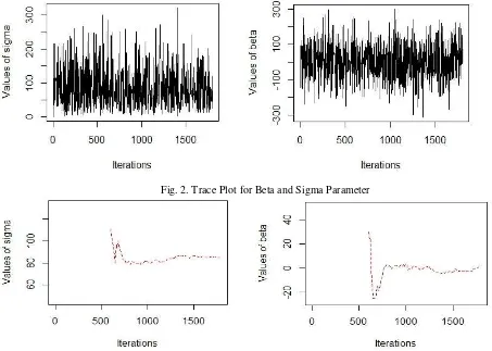
The results of cluster analysis were processed by using conditional Gibbs by inputting predictor variables (X1, X2, X3, X4, X5, and X6) to obtain the following results:
Fig. 2. Trace Plot for Beta and Sigma Parameter
ISSN 1013-5316;CODEN: SINTE 8 Sci.Int.(Lahore),30(4),523-527 ,2018
Fig. 4. Autocorrelation Function Plot for Beta and Sigma Parameter
The convergence of the Markov chain was shown in the
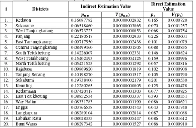
Table 2. Comparative Results of Pre-prosperous Family proportion with Direct and Indirect Estimation
i Districts Indirect Estimation Value
Direct Estimation Value
1. Kedaton 0.16087782 0.00000002832 0.165 0.0000720
2. Sukarame 0.06518460 0.00000003865 0.070 0.0001257
3. West Tanjungkarang 0.06573723 0.00000000853 0.068 0.0000754
4. Panjang 0.22180517 0.00000002933 0.226 0.0000601
5. East Tanjungkarang 0.09717550 0.00000002438 0.101 0.0001079 6. Central Tanjungkarang 0.08499460 0.00000001505 0.088 0.0000835 7. South Telukbetung 0.14226007 0.00000002331 0.146 0.0000824 8. West Telukbetung 0.15402493 0.00000004125 0.159 0.0000996 9. North Telukbetung 0.05421525 0.00000001292 0.057 0.0000816
10. Rajabasa 0.09869620 0.00000001819 0.102 0.0000908
11. Tanjung Senang 0.10198270 0.00000001517 0.105 0.0000790
12. Sukabumi 0.19738400 0.00000002179 0.201 0.0000530
13. Kemiling 0.12280265 0.00000000805 0.125 0.0000478
14. Kedamaian 0.07420417 0.00000001303 0.077 0.0000825
15. East Telukbetung 0.38852534 0.00000003337 0.393 0.0000351
16. Way Halim 0.08331783 0.00000001199 0.086 0.0000621
17. Enggal 0.03766538 0.00000004743 0.043 0.0001748
18. Langkapura 0.08289104 0.00000002814 0.087 0.0001088 19. Labuhan Ratu 0.08028335 0.00000005447 0.086 0.0001612
20. BumiWaras 0.08297342 0.00000001527 0.086 0.0000910
Based on the table 2, the estimated value of the proportion of each district by using the indirect estimator had a smaller value as it was compared with the estimated value of the proportion of each district by using the direct estimator. For the indirect estimator, the largest proportion value was 0.38852534. It meant that the proportion of the pre-prosperous family was 38.85% and it was in East Telukbetung . Moreover, the smallest proportion value was 0.03766538. It meant that the proportion of the smallest pre-prosperous families was 3.76% and it was in Enggal.
The average proportion of low-income families in Bandar Lampung was 0.11985 or 11.985%.
When the estimated proportion value was compared by the indirect estimator and the estimated value proportion was also compared by the direct estimator, a bias value ranges from 0.002 to 0.005. Based on the value of the bias, we knew that the value of estimated proportion between direct and indirect estimators had adjacent-tended values. If it is presented in Figure form, it appeared as follows:
Sci.Int.(Lahore),30(4),523-527 ,2018 ISSN 1013-5316;CODEN: SINTE 8
July-August
Fig.5. The Result of Comparison of Direct and Indirect Estimated Proportion
Based on the Figure 5, it was seen that the value of the estimated proportion between direct and indirect estimators showed the same tendency value. However, the value of the indirect assumption resulted a smaller value when it was compared to the value of the direct guess.
4. CONCLUSION
This study concludes that the proportion estimation with the indirect method is better than the direct method because the indirect assumption gives smaller standard deviation value.
REFERENCES
[1] Rao, J.N.K. (2003).Small Area Estimation. New York: John Willey and Sons.
[2] Neil R. Ver Planck, Andrew O. Finley, John A. Kershaw Jr., Aaron R. Weiskittel,Megan C. Kress, (2018). Hierarchical Bayesian Models for Small Area Estimation of Forest Variables Using LiDAR. Journal of Remote Sensing of Environment, 204, 287-295.
[3] Liu, B., Lahiri,P., and Kalton, G. (2014). Hierarchical Bayes Modeling of Survey-Weighted Small Area Proportions. Journal of Survey Methodology, 40, 1-13.
[4] BKKBN. http://aplikasi.bkkbn.go.id/mdk/Batasan MDK.aspx, Retrived 4 May, 2017.
[5] Carlin, B. P., and Chib, S. (1995). Bayesian Model Choice via Markov Chain Monte Carlo Methods Journal of the Royal Statistical Society. Series B (Methodological), 57(3), 473-484.
[6] Gelman, A., John B. Carlin, Hal S. Stern, David B. Dunson, Aki Vehtari, and Donald B.R . (2013). Bayesian Data Analysis, (3rd ed.), New York: Chapman & Hall/CRC.