STATISTICAL MODEL AND PREDICTION OF PINEAPPLE PLANT WEIGHT

(1)

STATISTICAL MODEL AND PREDICTION OF PINEAPPLE PLANT

WEIGHT

Mustofa Usman1, Faiz A. M. Elfaki3,*, Wamiliana1, Fauzan2, and Jamal I Daoud3

1_{Department of Mathematics, Faculty of Mathematics and Sciences, University of Lampung, Indonesia} 2_{Great Giant Pineapples Company, Lampung, Indonesia}

3_{Department of Sciences, Faculty of Engineering, IIUM, P.O.Box 10, 50728 Kuala Lumpur, Malaysia}

*Corresponding author e-mail: faizelfaki@yahoo.com; faizelfaki@iium.edu.my

ABSTRACT: In the Great Giant Pineapples Company, the problem of prediction of weight of fruits at harvest has become a long critical problem for the planning, cannery and marketing. The company has been trying for a long time to find the best method to predict the production of pineapple weight per hectare by using the information of plant weight. It is well known that the fruit weight has linear relationship with the pineapples plant weight. In this study, the modeling and prediction of pineapples plant weight will be discussed based on some factors. The experiment have been conducted in four difference locations and cultivar classes and varieties, namely location 094D with cultivar class Medium Crown and variety GP1, location 126C with cultivar class Medium Crown and variety GP1, location 158H with cultivar class Small Crown and variety GP1and in location 576D with cultivar class Medium Crown and variety GP1. The age of plants are 15 months of age. From each location 40 data has been taken by method of systematic random sampling. Than from each datum the plant weight (W) in kg, number of perfect leaves (NPL), the length of the longest leaf (LLL) in cm, and the width of the longest leaf (WLL) in cm are measured. From the analysis the plant weight best predicted by using variables NPL, LLL, and WLL in all locations.

Keywords: Plant Weight; NPL; LLL; WLL; Location; Regression Analysis; Model Comparison. 1. INTRODUCTION

In the Great Giant Pineapples Company, the problem of prediction of weight of fruits at harvest has become a long critical problem for the planning, cannery and marketing. In a modern pineapple farm or plantation, a primary objective is to schedule fruit production to make efficient use of resources and labor and to provide a regular and manageable supply of fruit to the fresh fruit market or the cannery. Scheduling of fruit harvest is approximately set at the time of planting. Planting material should be graded by size and type so that the planting material in a given field is as uniform as possible. Without this initial uniformity, it is difficult to assess how plants are developing and also to establish forcing and approximate harvest dates. If planting is done during periods with little or no rainfall, plants should be irrigated at least a few times if water and equipment are available. Irrigation helps get plants off to a quick and uniform start. Any variation that is introduced into the field at the time of planting is accentuated over time, which makes it difficult to assess the progress of growth over time and to schedule forcing to obtain a fruit of marketable size at harvest [1]. Many experiments and research has been conducted to develop a method for the estimation of the weight of pineapple fruits at harvest, this being one of the elements of major importance in the forecast of short-term production [2,3,4,5,6] by using simple linear regression found that fruit weight is positively correlated with increasing solar irradiance. In [7] authors conducted an experiments which has the final objective to identify the part of the plant which can be utilized for the establishment of prediction methods for the final weight of fruits and possible loss of production. Studies on the vegetative and reproductive components were also carried out. The diameter and height of the inflorescence and peduncle are fundamental elements of the plant better related to the final weight of fruits and can be used in the estimation method in the same way they should be used as variables in the regression analysis method. The final weight of fruits, together with the population, allows for a precise

prediction in the production of an area using a simple equation, with results which are economically and operatively more feasible. Estimates of plant weight made before the date of forcing to provide information about the progress of growth, i.e. are plants developing normally or is some unrecognized problem delaying growth. If the estimated plant weight indicates that plant growth is ahead of or behind what would normally be expected, forcing of plants can be rescheduled based on that information. If growth is progressing normally, forcing can occur on schedule, fruit harvest date can be predicted with reasonable accuracy, and the yield will also meet expectations. Many studies [4] have shown that fruit weight at harvest is highly correlated with

plant weight, plant leaf number and even ‘D’ leaf weight. D -leaf is the longest -leaf measured at the time of forcing [8]. Elsewhere [9] others separated pineapple leaves into categories based on their similarity in size and age. The ‘D’ group of leaves were the longest on the plant. Over time it

become common practice to apply the term ‘D-leaf’ as the

tallest leaf on the plant. As pineapple plants grow, ‘D’ leaves

get progressively longer and heavier and ‘D’ leaf weight at the time of forcing was highly correlated with fruit weight at

harvest for ‘Baronne de Rothschild’ but less well correlated for ‘Smooth Cayenne’ [10]. Others [8] recently reported that

‘D’ leaf weight was used as a forcing index for various pineapple cultivars in three different countries. As was noted

for plant weight, the relationship between ‘D’ leaf weight or

length at forcing and fruit weight at harvest likely will not be the same for all cultivars or for all countries or locations. [9] separated pineapple leaves into categories based on their

similarity in size and age. The ‘D’ group of leaves were the

longest on the plant. Over time it become common practice to

apply the term ‘D-leaf’ as the tallest leaf on the plant.

Others [5], in their study showed that by using simple linear regression analysis there was a linear relationship between fruit weight and plant weight for all, but one of the genotypes

(2)

very high fruit to- plant weight ratio of 0.60. Correlations between fruit weight and plant weight were carried out for each genotype to establish their relationship. The results indicated that the correlations were positive and significant in seven of the genotypes with the exception of A04-16. The correlation coefficients ranged from 0.41 to 0.86. [3] showed that there was a linear relationship between plant weight and fruit weight by using simple linear regression analysis. Plant or leaf weight at the time of forcing and fruit weight at harvest are generally highly correlated for a given variety of pineapple [2,3]. In the region near equator, where the environment is relatively uniform throughout the year, the correlation between plant or D-leaf at forcing and fruit weight at harvest might be expected to be high during most month of the year [11,10] showed that at a given plant weight leaf number varied with the cultivar.

In this present study, we will discuss how to predict the plant weight based on the information given by number of perfect leaves(NPL), the length of the longest leaf (LLL) in cm, and the width of the longest leaf (WLL) in cm. Multiple linear regression model will be used for the modeling of plant weight in the four different locations and cultivars, namely location 094D with cultivar class Medium Crown and variety GP1, location 126C with cultivar class Medium Crown and variety GP1, location 158H with cultivar class Small Crown and variety GP1and in location 576D with cultivar class Medium Crown and variety GP1 and to find the best model we will use backward elimination method, namely to eliminate the variable that has the smallest t or F values of all the variables in the equation [12]. The next analysis is to compare the similar models from the result of the first step analysis above, and to compare the models will be used the multiple linear regression with dummy variables.

2. STATISTICAL MODEL AND ANALYSIS

To analysis the data, we used multiple regression analysis for each location in the experiment. For the cases in this study the general linear regression model can be written as:

i

Model (1) to model (4) written in the matrix form. Also, the model’s can be written in a compact form as

It is well known that under the Gauss Markov model, the best

linear unbiased estimate of the parameter β’s for the models

are ([13], [14], [15], [16]): significant, then we continue to test the parameters of interest in the models, namely partial test of the parameters. To test the model, we used the principle conditional error (For interesting discussion concerning this method can be seen in [17], [14].

Under the null hypothesis, F has F-distribution with q and n-p degrees of freedom.

If F-test for teting

H

0

:

H





c

is significant, the next step

is to decide why Ho is rejected. Of course of action might be to test each of the individual constrains

H

₀

:

h



_k



_i



0 ,

h

) separately using a t-test, it is also called partial test for parameters (Seber, 1976; Graybill, 1976). The test is given in the following form:

(3)

To compare the regression models which have the same independent variables, we use multiple regressions with dummy variables. The model is developed based on model which can be found in [12,4,18,19]. The model will be developed based on the results of analysis from model (1) to (4).

3.RESULTS AND DISCUSSION

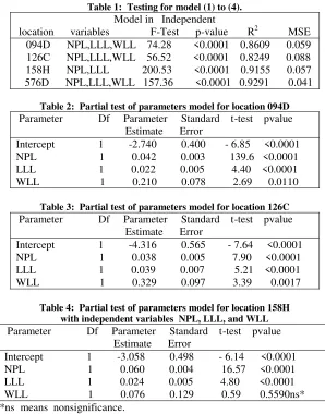
From the analysis data for model (1) to (4) by using SAS program, the results for testing the model in each location is given in Table 1.

From Table 1, the four models are very significant with P– value for each model <0.0001 and all Mean Square Error (MSE) for the four models relatively very small and very close to each other in the range between 0.041 to 0.088. For

model in location 094D, the plant weight 86.09% can be explained by NPL, LLL and WLL; For model in location 126C, the plant weight 82.49% can be explained by NPL, LLL and WLL; For model in location 158H, the plant weight 91.55% can be explained by NPL and LLL; For model in location 576D, the plant weight 92.91% can be explained by NPL, LLL and WLL.

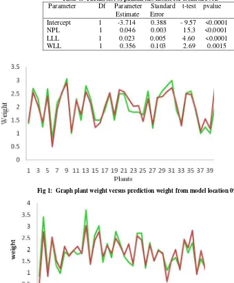
Partial test for each model (1) to (4) are given in Table 2 to Table 6 with Fig.1 to Fig. 4. For model (1) for location 094D given in Table 2, model (2) for location 126C given in Table 3, model (3) for location 158H given in Table 4 and Table 5, and model (4) for location 576D given in Table 6. Graph of relationship between plant weight from observation and plant weight from prediction from each significance model given in Fig.1 to Fig.4.

Table 1: Testing for model (1) to (4). Model in Independent

location variables F-Test p-value R2 MSE 094D NPL,LLL,WLL 74.28 <0.0001 0.8609 0.059 126C NPL,LLL,WLL 56.52 <0.0001 0.8249 0.088 158H NPL,LLL 200.53 <0.0001 0.9155 0.057 576D NPL,LLL,WLL 157.36 <0.0001 0.9291 0.041

Table 2: Partial test of parameters model for location 094D Parameter Df Parameter Standard t-test pvalue Estimate Error

Intercept 1 -2.740 0.400 - 6.85 <0.0001 NPL 1 0.042 0.003 139.6 <0.0001 LLL 1 0.022 0.005 4.40 <0.0001 WLL 1 0.210 0.078 2.69 0.0110

Table 3: Partial test of parameters model for location 126C Parameter Df Parameter Standard t-test pvalue Estimate Error

Table 4: Partial test of parameters model for location 158H with independent variables NPL, LLL, and WLL Parameter Df Parameter Standard t-test pvalue Estimate Error

Intercept 1 -3.058 0.498 - 6.14 <0.0001 NPL 1 0.060 0.004 16.57 <0.0001 LLL 1 0.024 0.005 4.80 <0.0001 WLL 1 0.076 0.129 0.59 0.5590ns* Note: *ns means nonsignificance.

Table 5: Partial test of parameters model for location 158H with independent variables NPL and LLL.

Parameter Df Parameter Standard t-test pvalue Estimate Error

(4)

Table 6: Partial test of parameters model for location 576D Parameter Df Parameter Standard t-test pvalue Estimate Error

Fig 1: Graph plant weight versus prediction weight from model location 094D

Plants

Fig 2: Graph plant weight versus prediction weight from model location 126C

(5)

Fig 4: Graph plant weight versus prediction weight from model location 576D

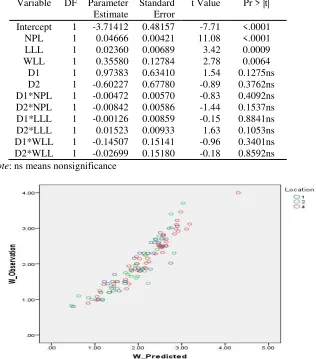
Table 7: Table Anova for testing model (9) Source Df Sum of Mean F-test p-value Square Square

Model 11 50.249 4.568 72.94 <0.0001 Error 108 6.763 0.062

C. Total 119 57.013 Note : R2 = 0.8814

Table 8: Anova Table for partial test for model (9). Variable DF Parameter

Estimate

Standard Error

t Value Pr > |t|

Intercept 1 -3.71412 0.48157 -7.71 <.0001

NPL 1 0.04666 0.00421 11.08 <.0001

LLL 1 0.02360 0.00689 3.42 0.0009

WLL 1 0.35580 0.12784 2.78 0.0064

D1 1 0.97383 0.63410 1.54 0.1275ns

D2 1 -0.60227 0.67780 -0.89 0.3762ns

D1*NPL 1 -0.00472 0.00570 -0.83 0.4092ns

D2*NPL 1 -0.00842 0.00586 -1.44 0.1537ns

D1*LLL 1 -0.00126 0.00859 -0.15 0.8841ns

D2*LLL 1 0.01523 0.00933 1.63 0.1053ns

D1*WLL 1 -0.14507 0.15141 -0.96 0.3401ns

D2*WLL 1 -0.02699 0.15180 -0.18 0.8592ns

Note: ns means nonsignificance

(6)

From the results of analysis above, model for location 094D, location 126C and location 576D have the same independent variables, namely NPL, LLL and WLL, while the model for location 158H the best model depend on the independent variables NPL and LLL only (Table 4 and Table 5). For comparison of these three models which have the same independent variables, namely model for locations: 094D, 126C and 576D we use multiple regression with dummy variables. The model as suggested by [12], [18], [19] can be written as follow: that the model (9) is very significance with overall F-test is 72.94, P-value <0.0001 and R2 = 0.8814 which means that 88.14% the variation of plant weight in the three locations can be explained by the model. The Anova table for the test is given Table 7 and 8.

To investigate the behavior of the relationship among the three models, we investigate the parameter for the dummy variable, namely the parameters β4to β11 in model (9).

For testing whether the models (1), (2) and (4) are equal. We use to test Ho : βL1o =βL2o = βL4o , Ho : βL11 =βL21 = βL41 ,

Ho : βL12 = βL22 = βL42 and Ho : βL13 =βL23 = βL43 and all

these null hypotheses are equivalent to the null hypotheses in model (9) as follow:

generally, all Ho are not rejected, therefore we can conclude that the model (1), (2) and (4) are not significantly different.

3. CONCLUSION

From the analysis data we can conclude that number of perfect leaves (NPL), the length of the longest leaf (LLL) in cm or D-leaf, and the width of the longest leaf (WLL) in cm can be used to predict the plant weight. Analysis for model (1), (2) and (4) shows that the relationship is positive and the models are very significance (P-value < 0.0001). In Model longest leaf or D-leaf. The graph for modification model (3) is given in Fig.3. The results of analysis for comparison model (1), (2) and (4), shows that they are not significantly different and the graph for the plants weight and its prediction by using model (9) for data from location 094D, location

[1] Pineapple News. Issue Newsletter of the

Pineapple Working Group, International Society for Horticultural Science , Issue 15 (2008).

[2] Bartholomew,D.P. and Paull, R.E., Pineapple

fruit set and development. In: Monselise, S.P.(ed.) Hanbook of Fruit Set and Development. CRC Press, Boca Raton, Florida, p. 371-388 (1986).

[3] Malezieux, E. Dry Matter accumulation and yield elaboration of pineapple in Cote d’Ivoire. Acta Horticulture 334: 149-157 (1993).

[4] Wee, Y.C., Tay,T.H., and Chiew,K.S. Correlation studies of leaf characteristics with fruit size in the Singapore Spanish pineapple. Malay Agric J .52:39-42 (1979).

[5] Chan, Y.K. and H.K. Lee. Performance of F1

pineapple hybrids selected for early fruiting, J. Trop. Agric. and Fd. Sc. 27(1): 1–8 (1999).

[6] Bartholomew, D.P. and Malézieux, E. Pineapple. In: Schaffer, B. and Anderson, P. (eds) Handbook of Environmental Physiology of Fruit Crops, Vol. II. CRC Press, Boca Raton, Florida, pp. 243–291(1994).

[7] García,H.D., and Consuegra R.M. Determination of the variables to use in the prediction of the pineapple production to cultivate Cayena Lisa. ISHS Acta

Horticulturae 666: _IV _{International} _Pineapple

Symposium, (2005).

(7)

[9] Sideris, C.P. and Krauss, B.H. The Classification and nomenclature of groups of pineapple leaves, section of leaves and section of stems based on morphological and anatomical differences, Pineapple Quarterly 6. 135-147 (1936).

[10] Fournier, P., Soler, A. and Marie-Alphonsine,P.A.

Growth characteristics of the pineapple cultivars ‘MD2' and ‘Flhoran 41' compared with ‘Smooth Cayenne'. Pineapple News 14 :18-20 (2007).

[11] Bartholomew, D.P., Malezieux, E, Sanewski and Sinclair, E. Inflorescence and Fruit Development and Yield. In The pineapple: Botany, Production and Uses (ed: D.P. Bartholomew, R.E. Paull and K.G. Rohrbach), (2003).

[12] _{Weisberg, S.}_{Applied Linear Regression. New York:}

John Wiley & Sons (1985).

[13] Graybill, F.A. Theory and Application of Linear Model. California:Wadsworth &Brooks/Cole, (1976). [14] Seber, G.A.F. Linear Regression Analysis, New

York: John Wiley & Sons (1976).

[15] Rao, C.R. Linear Statistical Inference and Its Applications, New York: John Wiley & Sons (1973). [16] Theil, Henri. Principles of Econometrics. New

York: John Wiley & Sons (1971).

[17] Milliken, G.A. New Criteria for Estimability for Linear Models, Ann. Math.Statist. 42. 1588-1594 (1971). [18] Skvarcius, R., and Cromer, F. A Note on the use of

Categorical Vectors in Testing for Equality of two Regression Equations. The American Statistician, 25: 27-29 (1971).

[19] Neter, J., Waserman, W., and Kutner,M.H. Applied Linear Statistical Model: Regression, Analysis of Variance and Experimental Designs. Boston,MA: Irwin (1990).