SPREAD OF INDONESIAN GOVERNMENT’S BOND
Chandra Utama
Faculty of Economics, Catholic University of Parahyangan
Shela Selviana Agesy
Alumni of Faculty of Economics, Catholic University of Parahyangan
ABSTRACT
This study analyzes the roles of macroeconomic variables, which include interest rate (SBI), Consumer Price Index (IHK), Jakarta Composite Index (IHSG), money supply (JUB) and exchange rate (KURS) on yield spread of government bonds (YSI) in Indonesia. The study employs Error Correction Model (ECM) on Indonesian monthly data from January 2008 to December 2013. The study confirms that SBI and KURS significantly determine the YSI in the short run and the long run but money supply is significant only in the long run. However, YSI is not influenced by IHK and IHSG. Based on term structure of interest rate theory, the study finds that the expected future interest rate is determined by SBI, KURS, and JUB.
Keywords: Government bond, Yield spread, Macroeconomic variable
JEL Classifications: G100, E00
INTRODUCTION
Initially, the issue of government bond is used to meet the need of banking
recapitulation as a consequence of the 1997 economic crisis. Besides, it is also used to
cover the deficit of Government budget. If in 2000 the government debt was dominated
by loans from other countries in the form of bonds, in 2008, the proportion of government’s debts was 55% from the domestic sources (in the form of bonds) and the remaining 45% from overseas. Meanwhile, in 2013, the proportion of the government’s
domestic debt was 69% and 31% was from other countries (General Directorate of
1The author expresses his/her gratitude to Dr. Miryam B. Lilian Wijaya for the comment and input which is very helpful for this research.
Debt Management (DJPU) 2013). This development shows that there is a restructrization of the government’s debt from a loan into a better security since the
interest rate requirement, term of maturity, and date of interest payable are decided by
Indonesian Government.
Simultaneous bond issued by the government increases the outstanding (amount)
of the government bond in the domestic bond market. If in 2000 the total outstanding
of the government bond was Rp. 31.63 trillions, in 2008 it increased to Rp. 525.69
trillions. In fact, in 2013, the total outstanding of the government bond reached Rp.
995.25 trillions (Financial Service Authority (OJK) 2014). Henceforth, the development
of the government bond triggers the increase of outstanding of company bond, which in
2000, 2008, and 2013 was as much as Rp.19.89 trillions, Rp.72.98 trillions, and
Rp.316.74 trillions respectively.
As mentioned by Blanchard (2011), between one bond and another will be
different in two dimensions, i.e. default risk and maturity. The former risk obviously
appears only in company bonds whereas the latter also exists in the government bond.
Next, Blanchard (2011), FRBSF (2003), Wu (2001), Ang and Piazzesi (2001), and Evans
and Marshall (2001) mentioned that the second risk occurs due to the change of
macroeconomic variables which transform market expectations to the economy which
influences the investment output in the future. This market estimation in the future is
illustrated by yield curve or known as term structure of interest rate. Yield curve with
positive inclination demonstrates the estimated yield in the future and it will increase
and expand the economy. Meanwhile, if the opposite applies, the market foresees
economic deceleration.
Several studies have been conducted to find out the effect of macroeconomic
variables on the estimated yield in the future. To measure the estimation, yield spread
(the difference between bond yield and long and short maturity) is used. A study by
Fah (2011) in Malaysia using growth variable of PDB, inflation, interest rate, money
supply, production index, trade balance, exchange rate, and Malaysian government
variables affecting yield spread include GDP growth, money supply, industrial
production, and trade balance. In the meantime, a study conducted by Ahmad et al
(2009) found that consumer price index and interest rate have the most significant
impact on the yield spread movement change. Also, Min (1998) who analysed the determinants of bond’s yield spread in 11 developing countries from 1991 to 1995,
found that debt to GDP ratio, debt service ratio, net foreign assset, international
reserves to GDP ratio, inflation rate, oil price, and exchange rate significantly affect
yield spread in terms of liquidity, solvability, and macroeconomic variables.
Batten et al (2006) studied government bond in Pacific Asia International Market,
i.e. China, Korea, Malaysia, Thailand and Phillipines with benchmark of US Treasury.
They found that bond yield spread in Asian countries has a negative correlation with an
interest rate change. In addition, exchange rate and stock market variables have a
significant influence on the change in yield spread, of which Philippines is the only
country where the stock market is negatively correlated with yield spread, while
exchange rate is positively correlated with the yield spread. Finally, the study held by
Sihombing et al (2012) found that macroeconomic variables affecting yield spread in
Indonesia include consumer price index (IHK) and BI rate.
Based on the previous studies, this study aims to examine the effect of
macroeconomic variables (BI rate, IHK, IHSG, money supply, and exchange rate) on
yield spread. Yield spread is calculated using the difference of government bond yield in
3 year maturity (short term) and 10 year maturity (long term). The selection of the
government bond is conducted because the government bond is a benchmark for
company bonds (Bank of Indonesia 2006). In fact, the proportion of government bond
in 2013 in the Indonesian bond market was 75,9% (OJK, 2013). Next, the government
bond has a default risk close to zero and homogenous; thus, the remaining risk is the
maturity.
In the second part of the paper, it will discuss theoretical review used in this
study. Research methodology and model specification is discussed in the third part. In
THEORETICAL REVIEW
Yield Spread is the difference between bond and different maturities. Yield spread can be influenced by the bond’s characteristics (Fabozzi et al, 2010). Besides,
the movement of yield spread can also be affected by the shock that exists in the
macroeconomy (Fah, 2011). The shock in macroeconomy can make the yield spread
getting wider or smaller. In general, this yield spread is used by investors to determine
the expected interest rates as well as the economy in the future. The following are
several basic concepts which explain the relationship between macroeconomic variables
and yield spread.
The Interest Rate of the Central Bank
According to Blanchard (2011), bond price (Pt) is determined based on the cash
flow value that can be obtained from bond ( ) and interest rate ( ). The price of bond
can be explained below:
(1)
In equation (1), if the interest rate increases, the bond price will decrease, while
if the interest rate decreases, the bond price will increase. The longer the maturity, the
higher percentage of bond price change will be, provided the interest changes.
However, the current interest change and the expected interest rate in the future
determine how significant the bond price will change. Bond price is directly related to
yield of bond. Consequently, the short term interest rate and the estimated short term
interest rate in the future determine the amount of bond yield in different tenors.
According to Blanchard (2011), the decrease of interest rate results in the
decrease of short term bond yield. Market actors estimate that in the long run, the
short term interest will return to the initial point, so the long term bond yield will be
higher than the short term more than the usual condition. The decrease of interest
predict that long term interest will go down proportionally as the decrease of the short
term, yield spread will not change.
Consumer Price Index
Consumer price index (IHK) is an index which measures the average price of
goods and services, whereas the percentage of its change is called inflation. Investors
who invest with certain risks will set a target on the real yield ( from their
investment. The real yield value is determined by the amount of its yield’s nominal
( ), inflation expectation, ( and other factors ( ); thus, it can be written as:
(2)
To simplify it, it is assumed that is constant, so the equation (2) is rewritten as
(3)
(4)
Equation (4) shows that the bigger the , the bigger the (which is asked by
investors). Based on the current inflation rate ( investors will the quantity of in
the future. When there is an increase in the IHK, short term will increase. If investors
expect that the common price will return in a long run, the yield spread will decrease.
In contrast, if investors estimate that the current price represents the future price, the
long term yield will also go up proportionally, so the yield spread will not be affected.
Jakarta Composite Index (IHSG)
In investing, investors take into account the rate of return and risk and avoid risk
(risk averse). Stocks basically have higher risk than bonds, even though they promise a
higher return. Investment portfolio made by investors is explained as follows (Handa
2009)
Where expected result of portfolio, E( , is determined by the average expected result
from stock, , and bond, times the proportion of each asset in portfolio,
and . Meanwhile, the estimated risk of portfolio which is measured by the root of the
varians portfolio ( ) can be written as
(6)
Where and are the standard deviations of stock, and is the estimated
correlation between stock and bond.
If stock return increases due to an increase in price, the maximum portfolio
composition for investors alters because investors raise the stock proportion in their
portfolio. The increasing stock demand leads to a decline in bond demand and price, so
the yield increases. This increasing yield is a short term yield. When in a long run,
investors expect that the stock market will be normal, the yield spread will go down on
the opposite side. If investors estimate that stock price increase keeps happening
proportionally, the yield spread will remain the same. The estimated stock return in a
term is usually arranged based on the current change in stock price.
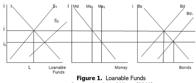
Money Supply
Money supply determines the amount of saving that can be invested. Economic
equilibrium occurs when saving is equal to investment, I=S. In figure 1, it is shown
when there is an increase of money offer, the movement of curve Ms1 to Ms2, results in
overfunding in the society, so saving rises, demonstrated by the shifting curve S1 to S2.
Overfunding owned by the society leads to the increasing demand of securities
including bond, shown by the displacement of curve Bd1 to Bd2. When demand for
obligation rises, the price of obligation will also increase, and yield will decrease. If the
market players predict that in a long run that money supply will go back to normal, the
Figure 1. Loanable Funds Source: Lewis and Mizen (2000)
Holding Obligation
In holding an asset (i.e. oligation), investors will have to face two choices; they
are holding domestic obligation or holding foreign obligation. To determine this
investment decision, investors rely on the expected exchange rate. Whether the
exchange rate in the future will be depreciated or appreciated will affect return
obtained by investors.
Investors have to choose between domestic obligation or foreign obligation. If
they buy the domestic obligation, they will get domestic yield as much as whereas if
they buy foreign obligation, they will receive yield as much as times the current
exchange rate, , divided by the expected exchange rate in the future, . This
condition is called interest rate parity which is written as the following:
(7)
If the domestic currency suffers from depreciation, the demand for domestic obligation
will decline, so the short term yield will increase. If in the long run, the exchange rate is
predicted to recover, the yield spread decreases. In contract, if the long term exchange
rate will proportionally turn to the current change, the yield spread does not change.
The data used in this study are monthly time series from January to 2008 to
January 2013. To obtain the yield spread, this study uses the Indonesian government
bond with 10 year and 3 year maturity. Meanwhile, the secondary data include monthly
BI rate (SBI), Consumer Price Index (IHK), Jakarta Composite Index (IHSG), money
supply (JUB), and exchange rate (KURS). These secondary data are obtained from Bank
of Indonesia, PT Dana Reksa, and Central Bureau of Statistics.
Prior estimating the long and short term effect of macroeconomic variables on
yield spread, the empirical model test is conducted using the methods of Akaike
Information criteria (AIC) and Final Prediction Error (FPE). Meanwhile, the test of
stationary level as well data integration of first difference is conducted using the
Augmented Dickey-Fuller (ADF) test. The existence of cointegration model, which is the
requirement in the ECM model, is estimated by the Johansen Cointegration. To come up
with residual value as the Error Correction Term (ECT) in the ECM model, this study
uses residual from the long term model by employing Ordinary Least Squares (OLS). To
find out the short term influence of macroeconomic variables on yield spread, ECM
model is used. Once the long term and ECM model are estimated, a classical
assumption test of multicolinearity and heteroscedasticity are conducted using the test
of White-heteroscedastcity, while the autocorrelation is tested using the Durbin-Watson.
Meanwhile, to test the heteroscedasticity in the ECM model, the
White-heteroscedasticity and autocorrelation tests are conducted using Breusch-Godfrey Serial
Correlation LM test.
Model Specification
To find the ECT value in the ECM, the following regression model in equation (8) is
applied
. (8)
In equation (8), the spread of the government bond, , is determined by BI rate,
, consumer price index, , Jakarta Composite Index, , money supply (M2),
term (residual) which, in the ECM model, is used as the ECT. Equation (8) also
demonstrates the long term effect of macroeconomic variables on yield spread.
Once the residual value of equation (8) is obtained, the ECM is estimated. ECM
used in this study can be arranged as
(9)
Where D represents the first difference from the variables. In the meantime, the ECT
can be defined as
(10)
Therefore, the ECM can be rewritten into
(11)
and represent the short-term and long-term effects of the independent variables
on A good and valid ECM model is then expected to have a significant ECT
(Insukindro, 1991), which can be represented in the statistical test result on ECT
coefficient.
DISCUSSION AND ESTIMATION RESULT Empirical Model Test
The selection of model is an important measure in empirical modeling. Faults in
determining the correct function form lead to problems in specification and inconsistent
estimation parameters. In this case, this study employs the criteria test of Akaike
Information criteria (AIC) and Final Prediction Error (FPE) to select variables that will be
used in the model.
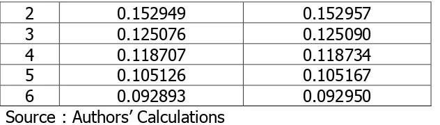
Table 1. AIC and FPE Calculation Result Step
2 0.152949 0.152957
3 0.125076 0.125090
4 0.118707 0.118734
5 0.105126 0.105167
6 0.092893 0.092950
Source : Authors’ Calculations
The result of model test is then compared from every step conducted. If the AIC
and FPE values of each step are smaller than the values from the the previous step, the
variables then can be used in the model. As presented in table 1, step 2 of the AIC and
FIP are smaller than those of step 1, then step 4 is smaller than step 3, while step 6 is
smaller than 5. Therefore, all the variables that will be used are proper in this study.
Unit Root Test
Unit root test to all variables used is necessary to meet the validity of ECM analysis. The
data is called stationary if they can fulfill these three elements, i.e. possessing a
constant average, a constant variance, and a constant covariance in every time unit
(Thomas, 1997). Table 2 presents the result of the unit root test using the Augmented
Dickey Fuller test at level phase. As presented in table 2, there is only one stationary
variable at the level phase, i.e. YSI variable (at the significance level of 5%) while SBI,
IHK, IHSG, JUB, and KURS are non stationary.
Table 2. Unit Root Test at the Level Phase
Variable ADF Value Probability Description
YSI -3.359419 0.0158 Stationary
As only one variable that stationary, we need to conduct the Augmented Dickey
Fuller phase at first-difference phase. As presented in table 3, at first difference, all the
variables used in this study are integrated (stationary) with a probability value of below
5%. The stationary condition at a similar degree is one of the requirements to see the
potential relationship and to avoid a spurious regression.
Table 3. Unit Root Test at the First Difference Phase
Variable ADF Value Probabilitty Description
Yield Spread -6.933019 0.0000 Stationary Interest Rate -3.313056 0.0180 Stationary
IHK -6.058594 0.0000 Stationary
IHSG -4.123914 0.0017 Stationary
JUB -10.23920 0.0001 Stationary
Exchange Rate -3.170666 0.0261 Stationary Source : Authors’ Calculations
Cointegration Test
Following the unit root test, the next step is conducting the cointegration test to
see the presence of long term relationship amongst variables. Johansen test of
cointegration test result is presented in table 4, showing that the Unrestricted Cointegration Rank Test (Trace) at α=5% shows at least 4 cointegration equation. As
for the test using Unrestricted Cointegration Rank Test (Maximum Eigenvalue), it
demonstrates that there are at least 2 cointegration variables.
Table 4. Cointegration Test Using Johansen Contegration Test
Unrestricted Cointegration Rank Test (Trace)
Hypothesized Trace 0.05
No. of CE(s) Eigenvalue Statistic Critical Value Prob.**
At most 4 0.174664 14.17174 15.49471 0.0783 At most 5 0.013333 0.926169 3.841466 0.3359
Trace test indicates 4 cointegrating eqn(s) at the 0.05 level * denotes rejection of the hypothesis at the 0.05 level **MacKinnon-Haug-Michelis (1999) p-values
Unrestricted Cointegration Rank Test (Maximum Eigenvalue)
Hypothesized Max-Eigen 0.05
No. of CE(s) Eigenvalue Statistic Critical Value Prob.**
None * 0.469853 43.78752 40.07757 0.0183
Max-eigenvalue test indicates 2 cointegrating eqn(s) at the 0.05 level
* denotes rejection of the hypothesis at the 0.05 level **MacKinnon-Haug-Michelis (1999) p-values
Source : Authors’ Calculations
Estimation Result of the Long Run Model
In equation (12) as follows, it can be seen the estimation result of long run
model. Then, the residual of this model will be used as ECT variable in ECM model.
Equation (12) indicates that SBI, IHSG, JUB, and KURS variables significantly
affect YSI (prob valua t-stat less than 5%), whereas IHK is insignificant. While the
influence of SBI and JUB are negative, that of KURS is otherwise. The F-statistic value
as much as 9.6487 or probability as much as 0.0001 means that independent variables
altogether affect the yield spread. Besides, R2 as much as 52,2% shows the ability of
the model in predicting the movement of YSI.
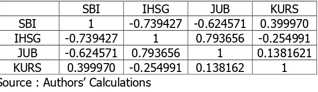
The first classic assumption test on equation (12) is multicolinearity, i.e. a
condition in which one or more independent variables have a liniar relation with each
other. One of the ways to analyze the existence of multicolinearity is by using
correlation matrix. If the correlation value between independent variables is more than
0,8, multicoliniarity can be a serious problem (Gujarati 2003, 359). In table 5, it is
shown that there is no correlation between independent variables which is bigger than
0.8; therefore, it can be concluded that there is no multocoliniarity issue in the model.
Table 5. Correlation between independent variables
SBI IHSG JUB KURS
SBI 1 -0.739427 -0.624571 0.399970 IHSG -0.739427 1 0.793656 -0.254991
JUB -0.624571 0.793656 1 0.1381621 KURS 0.399970 -0.254991 0.138162 1 Source : Authors’ Calculations
The next classical test is the heteroscedasticity test by using White
heteroskedastiscity test. This test is conducted by regressing the squared residual with
independent variables, squared independent variables, and multiplication between
n*R2. The criteria used are if 2 calculation is smaller than table 2, the zero hypothesis
which states that there is no heteroscadiscity in the model is accepted. Otherwise, if the
probability value is more than 5%, then there is no heteroscadiscity. The 2 value
calculated as much as 9.320891 is smaller than the critical value 2 as much as 31.4104
or Prob. Value as much as 0.9789 is bigger than 5%, so it can be concluded that there
is no heteroscedasticity.
The third assumption test in the long run model is the Durbin Watson. For
regression with 5 independent variables and 72 observations, obtained value of dl=1.58
and du=1.64, so the value of 4-du=2.36 and 4-dl=2.42. The value of DW-Stat. as much
as 0.915 indicates a positive autocorrelation. To improve the long term equation, the
Cochran-Orcutt iterative method is used next.
From equation13 it can be seen that the DW-Stat. value (1.842) is in the rejection
area between du=1,64 a nd 4-du=2,36, so it can be concluded that there is no
autocorrelation. Similarly, the calculated 2 value 18.146 is smaller than the 2 critical
value as much as 40.1132 or Prob. Value as much as 0.899 is more than 5% which
means that there is no heteroscedasticity.
t-stat: (2.288) (-3.241) (-0.930) (1.233) (-2.489)
(2.461)
Prob: (0.0255) (0.0019) (0.3561) (0.2221) (0.0154)
(0.0166)
+ 0.572 (AR1)
t-stat: (5.349)
R2 : 0.5979
F-stat: 15.859 Prob(F-stat): 0.000000
White Heteroscedasticity test: Obs*R-squared : 18.146 Prob.
Chi-Square(20):0.899
DW-Stat: .842
(13)
Based on the same equation, the SBI, JUB, and KUR significantly influence YSI
(the prob t-stat value below 5%), whereas IHK and IHSG are insignificant. The
conclusion of equation 13 is different from the long run equation (equation 12) which
shows the long term influence of IHSG. The effect of SBI and JUB is negative while
KURS is positive. The F-statistic value of 15.859 or probability 0.0000 indicates that all
independent variables altogether affect the yield spread. In addition, R2 demonstrates
that regression can explain the movement of yield spread as much as 59.79%. In this
regression that has been improved, it can be seen that the IHSG which previously
influences yield spread, becomes statistically non-influential.
ECM Estimation Result
After estimating the long run model (equation 13), the residual value from the
equation is used as ECT variable in ECM model. The following is the estimation result of
ECM. In the above ECM equation (equation 14), ECT coefficient, i.e. -0.367 is significant
(prob. value= 0.0077) so the ECM model is considered valid and there is a long term
relationship. It can be seen in the equation 14 that DSBI and DKURS significantly affect
yield spread (prob t-stat value below 5%) whereas IHK and IHSG are insignificant. SBI
and JUB have a negative impactwhile KURS is the opposite. The F-statistics (3,0416) or
probability (0,01112) indicates that independent variables altogether influence the yield
spread. Moreover, R2 proves that regression can explain the movement of yield spread
t-stat: (-0.876) (-2.071) (-.603) (0.803) (0.586)
Prob: (0.385) (0.0424) (0.5484) (0.4250) (0.5602)
t-stat: (2.110) (-2.750)
Prob: (0.0387) (0.0077)
R2 : 0.2219
F-stat: 3.0416 prob(F-stat): 0.01112
White Heteroscedasticity test:
Obs*R-squared : 20.0567 Prob. Chi-Square(20): 0.8284
Breusch-Godfrey Serial Correlation LM Test:
Obs*R-squared: 13.64997 Prob. Chi-Square(2): 0.0011
(14)
The following classical assumption test is the heteroscedasaticity test using White
heteroskedasticity test. In equation 14, it is informed that the calculated 2 value as
much as 20.0567 is smaller than the 2 critical vale as much as 31.4104 or Prob. Value
as much as 0.9789 is above 5%, thus it can be inferred that there is no
heteroscedascity.
In the ECM model, the Durbin-Watson test cannot be applied since DW statistic
will asymptotically be refracted to approach the value of 2 (Arief 1993 in Kurniawan
2004). For this reason, Breusch-Godfrey (BG) or better known as Lagrange Multiplier
(LM) Test is employed. The zero hypothesis in this test has no autocorrelation problem.
This test is done by regressing squared residual with independent variables. Next, the
the residual model with independent variables. Criteria used are if the calculated 2 is
smaller than table 2 , then the zero hypothesis stating that there is no autocorrelation
in the model is accepted, or if the prob. Is above 5% then autocorrelation does not
exist. For model in equation 14, it is known that the LM-test value or calculated 2 is as
much as 13.64997 and Prob. 0.0011, thus it can be concluded that there is an
autocorrelation. To better the long term equation, it is then used Cochran-Orcutt
iterative method. The improved ECM model is written below.
t-stat: (-0.777) (-2.406) (-0.780) (0.346) (0.276)
Prob: (0.4403) (0.0192) (0.4384) (0.7306) (0.7838)
t-stat: (2.552) (-2.931) (-1.861)
Prob: (0.0133) (0.0048) (0.0676)
R2 : 0.2692
F-stat: 3.1567 prob(F-stat): 0.006584
White Heteroscedasticity test:
Obs*R-squared :29.95090 Prob. Chi-Square(20): 0.7104
Breusch-Godfrey Serial Correlation LM Test:
Obs*R-squared: 5.36941 Prob. Chi-Square(3): 0.1467
(15)
In the ECM equation (equation 15), the coefficient of ECT variable, which is
-0.391, is significant (prob. value= 0.0048), so the ECM model is valid and has a long
term relationship in the ECM model. The value of ECT coefficient indicates that the 0.39
this month. In equation15, it can be seen that DSBI and DKURS significantly affect yield
spread (prob t-stat value below 5%), while IHK and IHSG are not significant. While the
effect of SBI is negative, that of KURS is positive. The improvement in the model does
not change the conclusion of the equation 14. The F-statistic value of 3.1567 or
probability 0.006584 indicates that all independent variables simultaneously influence
yield spread. Furthermore, R2 shows that regression can explain the movement of yield
spread as much as 29.95%.
It can also be informed from equation 15 that there is no heteroscesdacticity
problem. White heteroskedasticity test indicates the calculated 2 value 29,95 is smaller than
the 2 critical value 31.4104 or Prob. value 0,9789 is bigger than 5%. Meanwhile, the calculated
2 value in LM test which is as much as 5,36941 is less than the 2 critical value 7,8147 and
Prob. Value 0,1467 means that there is no autocorrelaion issue.
CONCLUSION
This study finds that the macroeconomic variables affecting yield spread in the long term are interest rate, active circulation, and exchange rate. In the meantime, variables influencing yield spread in the short term are interest rate and exchange. Consumer Price Index and stock market, on the other hand, do noo say that the increasing interest (y effects on the yield spread both in a short and long term.
Exchange rate also has a long term and short term balance with yield spread and has a positive sign. This condition is different from the initial prediction where the effect is negative. In investing, investors look at the return in the future, so the depreciation of rupiah, in fact, causes fund enter the market and rise the demand for bonds which can also be concluded that rupiah depreciation causes the market players, both in a short and long term, expect that there will be an increase in the market interest in the future. This positive relationship between exchange rate and yield spreadsimilar to findings by Batten et al (2006)
Unlike the inerest and exchange rate variables, active circulation only has negative long term effect. This situation is shown by the significant coefficient of active circulation effect in the long term model and the insignificance in the ECM model. This research result demonstrates that only in a long run, the rise in active circulation leads to an increase in bond yieldwith short maturity. This rise of active circulation makes the market players foresee a decrease of market interest in the future. The presence of active circulation effect on yield spread is the same as the research conducted by Fah (2011). The difference is, due to using OLS method, Fah (2011) does not indicate the short term effect of active circulation. Similarly, research by Batten et al. (2006) found the effect of exchange rate and interest on yield spread.
In this study, IHK variable illustrating real sector and IHSG describing the substitution of bond do not affect yield spread both in the long and short term. The non-existence influence of IHK is in line with the one conducted by Fah (2011), Ahmadet al. (2009), and Min (1998). On the contrary, this research result is against the study by Sihombing et al. (2012) which demonstrates the effect of IHK on yield spread in Indonesia. Meanwhile, the nonexistence of IHSG effect does not conform finding by Ahmad et al (2009) who found the long term and short term effect of interest, but only a long term effect of Malaysia stock price index (KLCI).
term structure of interest rate this research result proves that interest (BI rate), exchange rate, and active circulation affect market estimation regarding future interest.
REFERENCES
Ahmad, N., Muhammad, J., & Masron, T.A. (2009). Factors Influencing Yield Spreads Of The Malaysian Bonds. Asian Academy of Management Journal.14.2. 95-114.
Batten, J.A., Fetherston, T.A., & Hoontrakul, P. (2006). Factors Affecting The Yields of Emerging Market Issuers: Evidence From The Asia-pasific region. Journal of International Finance Markets, Institution and Money.16. 57-70.
Blanchard, O. (2011). Macroeconomics. (5th ed). Pearson.
Direktorat Jenderal Pengelolaan Utang. (2014). Buku Saku Perkembangan Utang Negara edisi
Januari 2014. Diunduh pada 23 Juni 2014 dari
http://www.djpu.kemenkeu.go.id/index.php/page/loadViewer?idViewer=3800&action=d ownload
Direktorat Jenderal Pengelolaan Utang. (2014). Laporan Analisis Portfolio dan Risiko Utang
Tahun 2013.Diunduh pada 23 Juni 2014 dari Market. International Journal of Humanities and Social Science. 1.5.
Federal Reserve Bank of San Francisco (FRBSF). (2003). What The Yield Curve Move?,FRBSF Economic Letter. Diunduh pada 7 Juli 2014 dari http://www.frbsf.org/economic-research/publications/economic-letter/2003/june/what-makes-the-yield-curve-move/ Gujarati, D.N. (2003). Basic Econometrics.4th edition. New York: Mc-Graw Hill.
Handa, J. (2009). Monetary Economics.2ndedition. London: Taylor & Francis Group.
Lnsukindro (1991). Regresi Linear Lancung dalam Analisa Ekonomi : Studi Kasus Permintaan Deposito Dalam Valuta Asing di Indonesia, Jurnal Ekonomi dan Bisnis Indonesiavolume 1 No.1
Kurniawan, T., (2004), Determinan Tingkat Bunga Pinjaman di Indonesia Tahun 1983-2002,
Buletin Ekonomi Moneter dan Perbankan, Bank Indonesia.
Lewis, M.K., & Mizen, P.D. (2000).Monetary Economics. New York: Oxford.
Min, G.H. (1998). Determinants Of Emerging Market Bond Spread: Do Economic Fundamentals
Matter. Diunduh pada 30 Januari 2014 dari
Otoritas Jasa Keuangan. (2014). Statistik Pasar Modal: Januari 2014. Diunduh pada 3 Juli 2014 dari http://www.ojk.go.id/januari-minggu-1-2014
Sihombing, P. et al (2012). Analisis Pengaruh Makroekonomi Terhadap Term Structure Interest Rate Obligasi Pemerintah (SUN) Indonesia.Jurnal Pasar Modal dan Perbankan.1.2. 103-114