Optimal monetary policy in a new Keynesi

Optimal Monetary Policy in a New Keynesian Model with

Habits in Consumption

∗

Campbell Leith

Ioana Moldovan

Ra

ff

aele Rossi

University of Glasgow

December 15, 2008

Abstract

While consumption habits have been utilised as a means of generating a hump-shaped output response to monetary policy shocks in sticky-price New Keynesian economies, there is relatively little analysis of the impact of habits (particularly, external habits) on optimal policy. In this paper we consider the implications of ex-ternal habits for optimal monetary policy, when those habits either exist at the level of the aggregate basket of consumption goods (‘superficial’ habits) or at the level of individual goods (‘deep’ habits: see Ravn, Schmitt-Grohe, and Uribe (2006)). Ex-ternal habits generate an additional distortion in the economy, which implies that theflex-price equilibrium will no longer be efficient and that policy faces interest-ing new trade-offs and potential stabilisation biases. Furthermore, the endogenous mark-up behaviour, which emerges when habits are deep, can also significantly af-fect the optimal policy response to shocks, as well as dramatically affecting the stabilising properties of standard simple rules.

• JEL Codes: E30, E57 and E61

• Key Words: consumption habits, nominal inertia, optimal monetary policy

1

Introduction

Within the benchmark New Keynesian analysis of monetary policy (see, for example, Woodford (2003)), monetary policy typically influences the economy through the impact of interest rates on a representative household’s intertemporal consumption decision. It has often been felt that the purely forward-looking consumption dynamics that such ba-sic intertemporal consumption decisions imply, are unable to capture the hump-shaped output response to changes in monetary policy one typically finds in the data. As a

means of accounting for such patterns, some authors have augmented the benchmark model with various forms of habits effects in consumption. The habits effects can either be internal (see for example, Fuhrer (2000), Christiano, Eichenbaum, and Evans (2005), Leith and Malley (2005)) or external (see, for example, Smets and Wouters (2007)) the latter reflecting a catching up with the Joneses effect whereby households fail to internalise the externality their own consumption causes on the utility of other house-holds. Both forms of habits behaviour can help the New Keynesian monetary policy model capture the persistence found in the data (see, for example Kozicki and Tinsley (2002)), although the policy implications are likely to be different. More recently, Ravn, Schmitt-Grohe, and Uribe (2006) offer an alternative form of habits behaviour, which they label ‘deep’. Deep habits occur at the level of individual goods rather than at the level of an aggregate consumption basket (‘superficial’ habits). While this distinction does not affect the dynamic description of aggregate consumption behaviour relative to the case of superficial habits, it does render the individual firms’ pricing decisions intertemporal and, in the flexible price economy considered by Ravn, Schmitt-Grohe, and Uribe (2006), can produce a counter-cyclical mark-up which significantly affects the responses of key aggregates to shocks.

While the focus of the papers listed above is on the dynamic response of economies which feature some form of habits, they do not consider the implications for optimal policy of such an extension. In contrast, Amato and Laubach (2004) consider optimal monetary policy in a sticky-price New Keynesian economy which has been augmented to include internal (but superficial) habits. Since the form of habits is internal (households care about their consumption relative to their own past consumption, rather than the consumption of other households), there is no additional externality associated with consumption habits themselves, and, given an efficient steady-state, the flexible price equilibrium in the neighbourhood of that steady-state remains efficient. Accordingly, as in the benchmark New Keynesian model, there is no trade-offbetween output gap and inflation stabilisation in the face of technology shocks and interesting policy trade-offs require the introduction of additional inefficiencies (such as mark-up shocks or a desire for interest rate smoothing).

In this paper we extend the benchmark sticky-price New Keynesian economy to include external habits in consumption, where these habits can be either superficial or deep. The focus on external habits implies that there is an externality associated with

and commitment. In addition to examining optimal policy, we also consider how the introduction of habits affects the conduct of policy through simple rules. We find that the introduction of deep habits can induce problems of indeterminacy, as the tightening of monetary policy can induce inflation through variations in mark-up behaviour, such that an interest rate rule which satisfies the Taylor principle (where nominal interest rates rise more than one for one with increases in inflation above target) may not be sufficient to ensure determinacy of the local equilibrium. We also consider whether or not there is a significant role for the output gap in an optimal simple rule given that our economy contains a major additional externality beyond that associated with nominal inertia.

The plan of the paper is as follows: in the next section we outline our model with deep and superficial habits. In section 3 we consider optimal policy under both commitment and discretion, where the policy-maker’s objective function is derived from a second order approximation to households’ utility. In section 4 we turn to our analysis of simple rules, considering both their determinacy properties and, for rules which can ensure determinacy, their ability to mimic optimal policy. Section 5 concludes.

2

The Model

The economy is comprised of households, two monopolistically competitive production sectors, and the government. There is a continuum of final goods that enter the house-holds’ consumption basket, eachfinal good being produced as an aggregate of a contin-uum of intermediate goods. Households can either form external consumption habits at the level of eachfinal good in their basket, Ravn, Schmitt-Grohe, and Uribe (2006) call this type of habits ‘deep’, or they can form habits at the level of the consumption basket - ‘superficial’ habits. Throughout the paper, we use the same terminology. Furthermore, we assume price inertia at the level of intermediate goods producers. We shall derive a general model, and note when assuming superficial or deep habits alters the behavioural equations.

2.1

Households

The economy is populated by a continuum of households, indexed by kand of measure 1. Households derive utility from consumption of a composite good and disutility from hours spent working.

Deep Habits When habits are of the deep kind, each household’s consumption basket,

X_tk, is an aggregate of a continuum of habit-adjusted final goods, indexed by i and of measure 1,

X_tk=

µZ 1

0

³

C_itk ₋θCit−1

´η−1 η

di

¶ η η−1

whereC_itk is householdk’s consumption of good iand Cit≡R₀1Citkdk denotes the

cross-sectional average consumption of this good. η is the elasticity of substitution between habit-adjustedfinal goods(η >1), while the parameterθmeasures the degree of external habit formation in the consumption of each individual goodi. Settingθto0 returns us to the usual case of no habits.

The composition of the consumption basket is chosen in order to minimize expendi-tures, and the demand forfinal goods is

C_itk =

µ

Pit

Pt

¶₋η

X_tk+θCit−1, ∀i

wherePtrepresents the overall price index (or CPI), defined as an average offinal goods

prices,Pt≡

³R1 0 P

1−η it di

´1/(1−η)

. Aggregating across households yields the total demand for goodi,i_∈[0,1],

Cit=

µ

Pit

Pt

¶−η

Xt+θCit−1. (1)

Due to the presence of habits, this demand is dynamic in nature, as it depends not only on current period elements but also on the lagged value of consumption. This, in turn, will make the pricing/output decisions of the firms producing these final goods, intertemporal.

Superficial Habits Habits are superficial when they are formed at the level of the ag-gregate consumption good. Households derive utility from the habit-adjusted composite goodXk

t,

X_tk=C_tk−θCt−1

where household k’s consumption, Ck

t, is an aggregate of a continuum of final goods

indexed byi_∈[0,1],

C_tk=

µZ 1

0

³

C_itk´ η−1

η di

¶ η η−1

with η the elasticity of substitution between them and Ct−1 ≡ R₀1Ctk−1dk the

cross-sectional average of consumption.

Households decide the composition of the consumption basket to minimize expendi-tures and the demand for individual good iis

C_itk =

µ

Pit

Pt

¶−η

C_tk=

µ

Pit

Pt

¶−η³

X_tk+θCt−1

´

wherePt≡³R₀1Pit1−ηdi

´ 1

1₋η

iis obtained by aggregating across all households,

Cit =

Z 1

0

C_itkdk

=

µ

Pit

Pt

¶−η

Ct. (2)

Unlike the case of deep habits, this demand isnotdynamic and thefinal goods producing

firms will face a static pricing/output decision.

Remainder of the Household’s Problem The remainder of the household’s

prob-lem is the same irrespective of whether or not habits are deep or superficial. Specifically, households choose the habit-adjusted consumption aggregate, X_tk, hours worked, N_tk, and the portfolio allocation, Dk

t+1, to maximize expected lifetime utility

E0

∞

X

t=0

βt

"¡

X_tk¢1−σ

1₋σ −χ

¡

N_tk¢1+υ

1 +υ

#

subject to the budget constraint

Z 1

0

PitCitkdi+EtQt,t+1Dt+1k =WtNtk+Dkt +Φkt −Ttk (3)

and the usual transversality condition. Et is the mathematical expectation conditional

on information available at time t, β is the discount factor(0< β <1), χ the relative weight on disutility from time spent working, and σ and υ are the inverses of the in-tertemporal elasticities of habit-adjusted consumption and work(σ, υ >0; σ6= 1). The household’s period-t income includes: wage income from providing labour services to intermediate goods producing firms WtNtk, dividends from the monopolistically

com-petitive firms Φk_t, and payments on the portfolio of assets D_tk. Financial markets are complete andQt,t+1 is the one-period stochastic discount factor for nominal payoffs. Ttk

are lump-sum taxes collected by the government. In the maximization problem, house-holds take as given the processes for Ct−1, Wt, Φkt, and Ttk, as well as the initial asset

positionDk₋₁.

The first order conditions for labour and habit-adjusted consumption are:

−χ

¡

N_tk¢υ

¡

Xk t

¢−σ =wt

and

Qt,t+1=β

Ã

X_t+1k X_tk

!₋σ

Pt

Pt+1

(4)

for consumption can be written as

1 =βEt

"Ã

X_t+1k Xk

t

!₋σ

Pt

Pt+1

#

Rt

where R−_t1 =Et[Qt,t+1] denotes the inverse of the risk-free gross nominal interest rate

between periods tand t+ 1.

2.2

Firms

In this subsection we consider the behaviour of firms. These are split into two kinds:

final and intermediate goods producing firms, respectively. In the case of the former, their behaviour depends upon the form of demand curve they face, which is dynamic in the case of deep habits, and static under superficial habits. Intermediate goods firms produce a differentiated intermediate good and are subject to nominal inertia in the form of Calvo (1983) contracts. This structure is adopted for reasons of tractability, allowing us to easily switch between superficial and deep habits. Additionally, combining optimal price setting under both Calvo contracts and dynamic demand curves would undermine the desirable aggregation properties of the Calvo model as eachfirm given the signal to re-set prices would set a different price dependent on the level of consumption habits their product enjoyed relative to otherfirms’. By separating the two pricing decisions we avoid reintroducing the history-dependence in price setting the Calvo set-up is designed to avoid.

2.2.1 Final Goods Producers

We assume that final goods are produced by monopolistically competitive firms as an aggregate of a set of intermediate goods (indexed byj), according to the function

Yit=

µZ 1

0 (Yjit)

ε−1

ε dj

¶ ε ε−1

, (5)

whereεis the constant elasticity of substitution between inputs in production(ε >1). Taking as given intermediate goods prices {Pjit}_j and subject to the available

tech-nology (5), firmsfirst choose the amount of intermediate inputs {Yjit}_j that minimize

production costsR₀1PjitYjitdj. The first order conditions yield the demand functions

Yjit=

µ

Pjit

Pm it

¶−ε

Yit, ∀j, ∀i, (6)

where Pm it ≡

³R1

0 Pjit1−εdj

´ 1

1₋ε

is the aggregate of intermediate goods prices in sector i

that this cost-minimisation problem takes the same form whether firms are faced with consumers whose habits are deep or superficial. However, their pricing decisions will differ across this dimension. We now examine the pricing decision offinal goods firms, dependent upon whether habits are deep or superficial.

Deep Habits When habits are deep,firms face the dynamic demand from households,

given by expression (1), and their profit maximization problem becomes intertemporal: the choice of price affects market share and future profits. Therefore, firms choose processes for Yit and Pit to maximize the present discounted value of expected profits,

Et

∞

X

s=0

Qt,t+sΦit+s, subject to this dynamic demand and the constraint that Cit =Yit.

Qt,t+siss-step ahead equivalent of the one-period stochastic discount factor in (4). The first order conditions for Yit and Pit are:

vit= (Pit−Pitm) +θEt[Qt,t+1vit+1] (7)

and

Yit=vit

"

η

µ

Pit

Pt

¶−η−1 _X t

Pt

#

, (8)

where the Lagrange multiplier vit represents the shadow price of producing an

addi-tional unit of the final good i. This shadow value equals the marginal benefit of addi-tional profits, (Pit−P_itm), plus the discounted expected payofffrom higher future sales,

θEt[Qt,t+1vit+1]. Due to the presence of habits in consumption, increasing output by

one unit in the current period leads to an increase in sales of θ in the next period. In the absence of habits, whenθ= 0, the intertemporal effects of higher output disappear and the shadow price simply equals time-t profits. The other first order condition in equation (8) says that an increase in price brings additional revenues, Yit, while

simul-taneously causing a decline in demand, given by the term in square brackets and valued at the shadow valuevit.

Superficial Habits Under superficial habits the profit maximization problem of the

final goodsfirms is the typical static problem wherebyfirms choose the price to maximize current profits,Φit = (Pit−Pitm)Yit, subject to the demand for their good (2) and under

the restriction that all demand be satisfied at the chosen price, Cit=Yit. The optimal

price is set at a constant markup,μ= _η−η₁, over the marginal cost,

2.2.2 Intermediate Goods Producers

The intermediate goods sectors consist of a continuum of monopolistically competitive

firms indexed by j and of measure 1. Each firm j produces a unique good using only labour as input in the production process

Yjit=AtNjit. (9)

Total factor productivity, At,affects all firms symmetrically and follows an exogenous

stationary process, lnAt = ρlnAt−1+εt, with persistence parameter ρ ∈ (0,1) and

random shocks εt∼iidN

¡

0, σ2 A

¢

.

Firms choose the amount of labour that minimizes production costs,(1−κ)WtNjit.

The subsidy _κ, financed by lump-sum taxes, is designed to ensure that the long-run equilibrium is efficient.1 The minimization problem gives a demand for labour Njit =

Yjit

Ajit and a nominal marginal costM Ct= (1−κ)

Wt

At,which is the same acrossfirms. (See

Appendix A for more details.) Nominal profits are expressed asΦjit≡(Pjit−M Ct)Yjit.

We further assume that intermediate goods producers are subject to the constraints of Calvo (1983)-contracts such that, with fixed probability (1−α) in each period, a

firm can reset its price and with probability αthefirm retains the price of the previous period. When a firm can set the price, it does so in order to maximize the present discounted value of profits,Et

∞

X

s=0

αsQt,t+sΦjit+s, and subject to the demand for its own

good (6) and the constraint that all demand be satisfied at the chosen price. Profits are discounted by thes-step ahead stochastic discount factor Qt,t+s and by the probability

of not being able to set prices in future periods.

Optimally, the relative price satisfies the following relationship:

P_jit∗ Pt

=

µ

ε ε₋1

¶ Et

∞

X

s=0

(αβ)s(Xt+s)−σmct+s¡Pit+sm

¢ε

Yit+s

Et

∞

X

s=0

(αβ)s(Xt+s)−σ

³

Pt+s

Pt

´−1¡

Pm it+s

¢ε

Yit+s

wheremct= MC_Ptt is the real marginal cost.

Pm

it represents the price at the level of sector i and is an average of intermediate

goods prices within that sector. Withαoffirms keeping last period’s price and (1₋α)

of firms setting a new price, the law of motion of this price index is:

(P_itm)1−ε=α¡P_itm₋₁¢1−ε+ (1₋α)¡P_jit∗ ¢1−ε.

This description of intermediate goods firms is the same irrespective of the nature of

habits formation.

2.3

The Government

The government collects lump-sum taxes which it rebates to intermediate goods pro-ducingfirms as subsidies, which ensure an efficient long-run level of output. There is no government spending per se. The government budget constraint is given by

κWtNt=Tt. (10)

In this cashless economy, monetary policy is conducted in optimal fashion, with the nominal interest rate being the central bank’s policy instrument. However, we also consider the consequences of the central bank adopting more simple forms of policy, such as Taylor-type interest rate rules, and explore how closely these simple policy rules come to the optimal.

2.4

Equilibrium

In the absence of sector-specific shocks or other forms of heterogeneity, final goods producers are symmetric and so are households. However, symmetry does not apply to intermediate goods producers who face randomness in price setting. There is a distribution of intermediate goods prices and aggregate output is therefore determined as (see Appendix B for details on aggregation)

Yt=At

Nt ∆t

. (11)

∆t≡

Z 1

0

³

Pjt

Pm t

´₋ε

djis the measure of price dispersion, which can be shown (see Wood-ford (2003), Chapter 6) to follow an AR(1) process given by

∆t= (1−α)

µ

P_t∗ Pm

t

¶−ε

+α(πm_t )ε∆t−1. (12)

Note that we have two measures of aggregate prices, a producer price index P_tm

and the usual consumer price indexPt, and consequently, there will be two measures of

inflation. We define: πm_t ≡ Ptm

Pm

t−1 andπt≡

Pt

Pt−1.Furthermore, the two inflation variables

are related according to the following relationship

πt=πmt

μ_t

μ_t−1, (13)

whereμ_t≡ Pt

Pm

t is the markup offinal goods producers. In the presence of deep habits,

of markups in the intermediate goods and final goods sectors and equals the inverse of the real marginal cost,mc−_t1 = Pt

MCt. It should be noted that when habits are superficial,

the mark-up in the final goods sectors is constant, μ_t =μ, and there is no longer any wedge between consumer price and producer price inflation.

Finally, the aggregate version of the household’s budget constraint (3) combines with the government budget constraint (10) and the definition of aggregate profits (Φt =

PtYt−(1−κ)WtNt) to obtain the usual aggregate resource constraint,

Yt=Ct. (14)

The equilibrium is then characterized by equations (11) - (14), to which we add the monetary policy specification (to be detailed in Sections 3 and 4 below) and the following set of equations:

Consumers:

Xt=Ct−θCt−1 (15)

−χN

υ t

X_t−σ =wt (16)

X_t−σ =βEt ∙

X_t+1−σ Pt Pt+1

¸

Rt (17)

Government:

κWtNt=Tt (18)

Intermediate goods producers:

(P_tm)1−ε=α¡P_tm₋₁¢1−ε+ (1−α)¡P_jt∗¢1−ε (19)

P_jt∗ Pt

=

µ

ε ε₋1

¶

K1t

K2t

(20)

where : K1t=Xt−σmctμt−εYt+αβEt£K1t+1πεt+1

¤

(21)

: K2t=Xt−σμ−tεYt+αβEt£K2t+1πε_t+1−1¤ (22)

mct= (1−κ)

wt

At

(23)

lnAt=ρlnAt−1+εt (24)

Final goodsfirms:

inter-mediate goods,

μ_t=μ. (25)

In contrast, when habits are deep and final goods firms face a dynamic demand curve for their product, the endogenous time varying mark-up is described by the following two equations (note that we have written the shadow price of producing final goods in real terms, i.e. ωt≡ _Pvt_t),

ωt=

µ

1₋ 1

μ_t

¶

+θβEt

"µ

Xt+1

Xt

¶−σ

ωt+1

#

(26)

Yt=ηωtXt. (27)

2.5

Solution Method and Model Calibration

In the absence of a closed-form solution, the model’s equilibrium conditions are log-linearized around the efficient deterministic steady state. The efficiency of the steady state, obtained through the subsidy allocated to intermediate goods producers, allows us to obtain an accurate expression for welfare involving only second-order terms.

In order to solve the model, we must select numerical values for some key structural parameters. Table 1 reports our choices, which are similar to those of other studies using a New Keynesian economy with habits in consumption. The model is calibrated to a quarterly frequency. We assume zero average inflation (π= 1) and an annual real rate of interest of 4%, which together imply a discount factor β of 0.9902. The risk aversion parameter σ is set at 2.0, while υ equals 0.252, and the relative weight on labour in the utility function χ is assumed to be 3.0. Consistent with the empirical evidence, the level of price inertia α is set at 0.75 and the degree of market power is 1.21, split approximately equally between the two monopolistically competitive sectors of our economy. The steady state value of the markup in the final goods sector is given as,μ=h1_{− (1}(1−₋θβ)_θ)ηi−1, and depends on both the elasticity of substitution betweenfinal goods η and the degree of habit formation θ. However, the impact of θ on the markup

μis minimal and we therefore set η=ε= 11. For the habit formation parameterθ, we use a benchmark value of0.65, which falls within the range of estimates identified in the literature3. However, we allowθ to vary in the [0,1)interval as we conduct sensitivity analyses of our results. Technology shocks are assumed persistent with persistence parameterρ= 0.9and standard deviation σA= 0.009. Finally, we set the subsidy rate κ so as to ensure an efficient steady state,κ = 1− 1

1−θβ

³

1 με−ε1

´

.

2

υis the inverse of the Frisch labour supply elasticity. While micro estimates of this elasticity are rather small, they tend not tofit well in macro models. Here, we follow the macroeconomic literature and choose a larger value of 4.0.

2.6

Log-linear Representation

Upon log-linearizing and combining the relevant equilibrium conditions, we obtain a system of equations which characterize the dynamics of the economy in the neighborhood of the efficient steady state. Firstly, we have the IS curve in terms of habit-adjusted consumption,

and the New Keynesian Phillips Curve (NKPC) written in terms of producer price inflation

b

πm_t =βEtbπmt+1+κ(mcct+bμt) (29)

where κ ≡ (1−αβ)(1_α −α) and it should be remembered that the markup, μ_t, is constant under superficial habits such that, _bμ_t = 0. In contrast, when habits are deep, the dynamic equation describing changes in the markup can be written as,

b

where the shadow value of producing another unit of afinal good subject to deep habits is given by,

b

ωt=Ybt−Xbt. (31)

And finally, we have the following expressions defining habit-adjusted consumptionXbt,

CPI inflation bπt (when habits are deep), and the real marginal costmcct:

In this section we consider the nature of optimal monetary policy in response to technol-ogy shocks, under both cases of commitment and discretion by the monetary authority. The central bank’s objective function is given by a second order approximation to the representative households’ utility (see Appendix E for details),

where δ _{≡ (1−θβ)(1}σ _−θ). The last line was obtained by replacing Xbt with its expression

in terms of output. The weights given to the various elements in the objective function are derived from basic preference parameters, and the presence of the term in inflation reflects the costs of price dispersion due to nominal inertia. It should be noted that this objective function applies whether or not habits are deep or superficial.

While this welfare measure has the same basic components (output and inflation) as the benchmark New Keynesian model (without externalities due to consumption habits), this welfare measure looks different, in that it does not contain a single “output gap”, defined as the difference between output and the flex-price level of output. However, the more complex term in the current set-up is conceptually similar. The output gap term in the standard analysis captures the extent to which output deviates from its efficient level (typically because of nominal inertia, rather than any other distortion). In a model with external habits, there is an additional externality which means that the

flexible price equilibrium is unlikely to be efficient, such that it is not possible to rewrite output in gap form. Nevertheless, it is possible to show that minimisation of the terms in square brackets is equivalent to implementing the social planner’s allocation. In other words, we are still trading off inflation control against minimising the deviation of the decentralised equilibrium to that which would be implemented by a benevolent social planner (see appendix D for the social planner’s problem).

We measure the welfare cost of a particular policy as the fraction of permanent consumption that must be given up in order to equal welfare in the stochastic economy to that of the efficient steady state,E P∞

t=0

βtu(Xt, Nt) = (1−β)−1u¡(1−θ) (1−ξ)C, N¢.

Given the utility function adopted, the expression forξ in percentage terms is

ξ =

"

1₋ [(1−σ)Υ]

1

1−σ

(1₋θ)C

#

×100,

whereΥ_≡(1₋β)W+χN_1+υ1+υ andW _≡EP∞

t=0

βtu(Xt, Nt) represents the unconditional

expectation of lifetime utility in the stochastic equilibrium.

3.1

Optimal Policy under Commitment

If the monetary authority can credibly commit to following its policy plans, it then chooses the policy that maximizes households’ welfare subject to the private sector’s optimal behaviour, as summarized in equations (28) - (34), and given the exogenous process for technology (see Appendix F for details of the policy problem under com-mitment). We analyze the implications of this policy in terms of impulse responses to exogenous technology shocks.

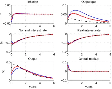
habits, policy would be loosened to ensure the flexible price equilibrium was recreated without generating any inflation (see Amato and Laubach (2004)).4 However, when habits are external, such that one household does not take account of the impact their increased consumption has on the utility of others, then with one policy instrument available, the monetary authority cannot simultaneously ensure output is at its efficient level and inflation is eliminated. Instead, while nominal inertia points to a relaxation of policy in the face of a positive technology shock to boost output, the consumption exter-nality suggests that the higher consumption this entails need not be desirable.5 Figure 1 shows that the optimal response of the economy to a positive persistent technology shock is a positive output gap and an initial decline followed by an increase in inflation (pluses indicate the benchmark calibration with θ= 0.65) when habits are superficial.

To achieve this outcome, the monetary authority reduces the nominal interest rate to boost demand to the socially optimal level. Because the policy is expansionary, we can implicitly say that the inefficiency due to price stickiness is dominating in this case. As the degree of importance of habits increases, inflation stabilisation remains the primary goal and the policy maker suffers a widening output gap due to the consumption externality.

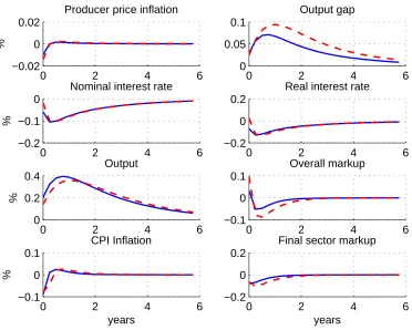
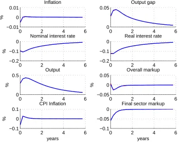
We turn to the case of deep habits in Figure 2. Holding the monetary policy response constant, we would expect the slackening of monetary policy to increase the discounted profits of final goodsfirms, encouraging them to cut current markups, generating con-sumption habits in their goods and thereby widening the output gap further. As a result, the optimal monetary response does not slacken real interest rates by as much in order to discourage the reduction in mark-ups. In fact, once the degree of habits passes a certain level, real interest rates actually rise initially, as policy makers seek to dampen the initial rise in consumption which imposes an undesirably externality on households. This can be seen in Figure 2, where solid lines depict impulse responses under the benchmark value of habits, θ= 0.65, and dash lines the responses under an alternative higher value of θ= 0.75.

3.2

Optimal Policy with Discretion

The previous sub-section examined policy under commitment. It is well known that not being able to commit to a time-inconsistent policy can give rise to a stabilisation bias in the New Keynesian economy whereby policy makers cannot obtain the most favourable tradeoffs between output gap and inflation stabilisation. In our economy with a consumption externality, there may be additional sources of stabilisation bias which make it interesting to assess the importance of having access to a commitment

4_{Of course, this is also the case in the New Keynesian model without habits - in the face of technology} shocks, the monetary policy maker can eliminate the output gap without generating inflation.

technology. Appendix F defines the inputs to the iterative algorithm used to compute time-consistent policy in Soderlind (1999).

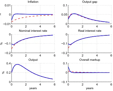
Figure 3 contrasts policy under discretion and commitment when habits are

super-ficial. Aside from failing to exploit the expectational benefits of price level control, the discretionary policy also fails to achieve the initial relative tightening of policy which mitigates the generation of undesirable habits effects. The desirability of undertaking the commitment policy emerges in the significantly different paths for inflation across commitment and discretion. The welfare cost of not being able to commit to future policies amounts to 0.016% of steady state consumption and it is 0.77% higher than under commitment, in the benchmark case of θ= 0.65.

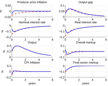
When we undertake the same comparison in the case of deep habits (see Figure 4), the time inconsistency problem is even more significant than in the case of superficial habits. This is because under deep habits there is a stronger desire to tighten policy initially in order to prevent an undesirable increase in consumption habits, exacerbated by the profit-maximising cuts in mark-ups by final goods producing firms. In fact, under commitment, interest rates actually rise initially if the extent of habits formation exceeds θ = 0.73. Since such a policy is designed to improve policy trade-offs in the future, it is not possible to engineer such a monetary tightening under time consistent policy. The costs of not having access to a commitment technology are correspondingly higher under deep habits, where the welfare costs under discretion are 1.98% higher than commitment, under the benchmark ofθ= 0.65.

4

Simple Rules

Having derived the optimal policy under commitment and discretion for our new Key-nesian economy with either superficial or deep habits, we now turn to consider the following simple monetary policy rule,

b

Rt=φπbπmt +φyYbtgap+φRRbt−1.

This is similar to that considered in Schmitt-Grohe and Uribe (2007), but with some differences noted below. Rbtis the nominal interest rate,πbmt is the rate of inflation in the

Wren-Lewis (2006)).6 We also include a term in the output gap rather than output itself. Schmitt-Grohe and Uribe (2007) demonstrate that a term in output plays no role in an optimally parameterised simple rule, and we wish to assess, in contrast to this

finding, whether there is a role for policy responding to a measure of the inefficiency in the level of output in an economy with a potentially large consumption externality.

In this section we begin by considering the determinacy properties of our simple rule, under both forms of habit formation. We then turn to consider the welfare maximising parameterisation of the rule, and assessing to what extent this can mimic the optimal policy under commitment described above.

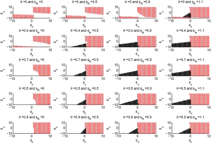
Figure 5 details the determinacy properties of this rule when habits are of the superfi -cial form. Each sub-plot details the combinations ofφ_π andφ_ywhich ensure determinacy (light grey dots), indeterminacy (blanks) and instability (dark grey stars). Moving from left to right across subplots increases the degree of interest rate inertia in the rule,φ_R, while moving down the page increases the extent of habits formation, θ. Consider the

first sub-plot in the top left hand corner withφ_R= 0andθ= 0, which re-states the sta-bility properties of the original Taylor rule. Here the importance of the Taylor principle is revealed as φ_π > 1 in combination with a non-negative response to the output gap is a sufficient condition for determinacy. Within this region there is limited scope for compensating for failing to fulfil the Taylor principle through increasing the positive re-sponse of the interest rate to the output gap, and there is slightly greater scope for using a more aggressive monetary policy response to compensate for a mildly negative interest rate response to the output gap. It is also interesting to note that a second region of determinacy exists where the interest rate rule fails to satisfy the Taylor principle, such thatφ_π <1, and the response to the output gap is strongly negative. This region is not often discussed in the literature, but is mentioned in Rotemberg and Woodford (1999). Typically, when monetary policy fails to satisfy the Taylor principle inflation can be driven by self-fulfilling expectations which are validated by monetary policy. However, when the output gap response is sufficiently negative there is an additional destabilising element in policy, which overturns the excessive stability generated by a passive mon-etary policy, implying a unique saddlepath where any deviation from that saddlepath will imply an explosive path for inflation.

As we move down the sub-plots in thefirst column of Figure 5 we increase the degree of superficial habits. This means that the output response to both policy and shocks is more muted as current consumption is increasingly tied to past levels of consumption. This has two effects on the determinacy properties of the basic Taylor rule. Firstly, a rule which satisfies the Taylor principle will do so even if the response to the output gap is increasingly negative. Secondly, the additional instability caused by adopting a

negative interest rate response to the output gap becomes insufficient to move a passive interest rate rule to a position of determinacy. Accordingly, the importance of the Taylor principle is enhanced when consumption is subject to superficial habits effects.

As we move across the page from left to right we increase the extent of interest rate inertia in the rule. In this case, as Woodford (2001) shows, the Taylor principle needs to be rewritten in terms of the long-run interest rate response to excess inflation, φπ

1−φ_R >1.

As a result, the determinacy region in the positive quadrant spreads further into the adjacent quadrants since a given level of instantaneous policy response to inflation φ_π

has a far greater long-run effect.

Finally, when we combine superficial habits effects with interest rate inertia, it be-comes possible to induce instability in our economy when the rule is passive, φπ

1−φR <1,

and the interest rate response to the output gap is negative, φ_y < 0. Essentially, the slow evolution of consumption under habits combined with interest rate inertia and a perverse policy response to output gaps and inflation serves to induce a cumulative instability in the model.

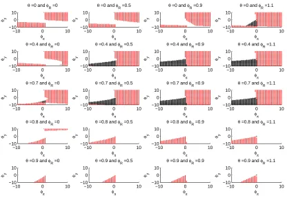
Figure 6 constructs a similar set of sub-plots when habits are of the deep, rather than superficial, kind. If the extent of habits formation is relatively low, the deter-minacy properties of the model are similar to those observed under superficial habits. However, when the degree of habits formation exceeds θ > 0.77, then there are some significant differences. Firstly, the usual determinacy region in the positive quadrant disappears and becomes indeterminant. This indeterminacy is linked to the additional dynamics displayed in the final goods sectors, where the markup is time-varying under deep habits formation. Suppose economic agents expect an increase in inflation. Given an active interest rate rule,φ_π >1, this will give rise to a tightening of monetary policy. Typically, such a policy would lead to a contraction in aggregate demand, invalidating the inflation expectations. However, in the presence of deep habits, the higher real interest rates will encourage final goods firms to raise current mark-ups as they dis-count the lost future sales such price increases would imply more heavily. If the size of habits effects is sufficiently large, then this increase in mark-ups can validate the initial increase in inflationary expectations, leading to self-fulfilling inflationary episodes and indeterminacy.

Furthermore, the region of instability identified under superficial habits, becomes determinate when combined with the excessive stability implied by endogenous mark-up behaviour, such that the only determinant rule in the presence of a large deep habits effect is where the rule is passive, φπ

1−φ_R <1,and the policy response to the output gap

is sufficiently strongly negative.

Optimal Rules Having explored the determinacy properties of the simple rule

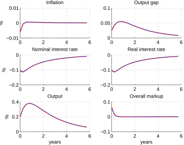
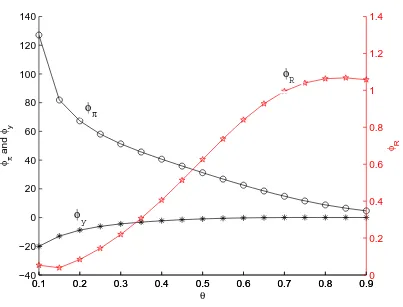
habits, we now turn to consider the optimal parameterisation of the rule in each case.7 In the case of superficial habits and under the benchmark value ofθ= 0.65, the optimal rule implies a lot of interest rate smoothing, with a strong positive response to inflation but a negative response to the output gap (φ_π = 18.47, φ_y = ₋0.09, and φ_R = 0.93). With this type of optimal monetary policy rule, the economy’s response to a technology shock essentially replicates the responses obtained under a full commitment policy, as shown in Figure 7. To explore the intuition underpinning this result, Figure 8 explores how the optimal policy rule parameters vary with the degree of habits formation,θ.

In the absence of habits effects, in a New Keynesian economy, a positive technology shock leads to a decrease in inflation and, due to the nominal inertia, an insufficiently large increase in output. Optimally, a decrease in the nominal interest rate stimulates demand by reducing the real interest rate. This can be achieved by having a very large coefficient on inflation relative to all other parameters, which essentially allows the simple policy rule to achieve the flex-price equilibrium with zero inflation and a zero output gap. As we introduce superficial habits effects, in the face of the same shock households overconsume and the output gap becomes positive suggesting that policy be tightened rather than relaxed. This trade-off, which is not present in the model without external habits, affects the optimal parameterisation of the simple policy rule. Specifically, as we increase the degree of habits formation, the optimal parameter on inflation in the simple rule falls and the extent of interest rate inertia increases. Furthermore, the negative coefficient on the output gap also falls, eventually turning positive.

A key feature of optimal policy under commitment is price level control where the optimal policy achieves expectational benefits in seeking to ensure that price level returns to base following any shock. As the degree of superficial habits formation is increased, this price level control can be achieved most effectively through a combination of interest rate inertia and output gap response. Consider the impact of the positive technology shock depicted in Figure 7. Essentially, the rule is able to maintain a cut in real interest rates, even when inflation is slightly positive (to undo the price level effects of the initial fall in inflation), by responding negatively to the persistent positive output gap and maintaining that stance for longer by increasing the amount of interest rate inertia. When the degree of habits formation becomes sufficiently large, the coefficient on the output gap becomes positive in order to reduce the initial relaxation of policy, and the degree of interest rate inertia is increased to ensure price level control.

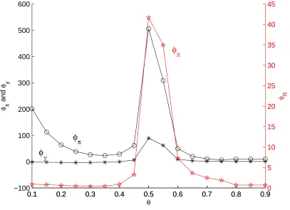
Figure 9 plots the optimal parameters of the simple rule, when the economy features an increasing level of deep habits formation. When habits are deep there is less of a desire to cut interest rates initially, to prevent final goods firms’ cutting their mark-ups and generating even greater consumption externalities. For relatively low levels

of habits, this implies a more muted response to inflation and output gaps. However, there is a surprising ‘blip’ in the optimal parameters for intermediate levels of the deep habits effect. At intermediate levels of deep habits this desire to tighten policy isfinely balanced against the need to avoid falls in intermediate goods inflation which induces undesirable increases in price dispersion. Despite the large rule parameters this implies, the rule still successfully mimics optimal policy under commitment, and the simple rule in all cases comes close to achieving the welfare levels observed under commitment - see Figure 10 for an illustration of impulse responses to a technology shock in the case of

θ= 0.5.

5

Conclusion

In this paper we considered the optimal policy response to technology shocks in a New Keynesian economy subject to habits effects in consumption. These effects were as-sumed to be external, such that one household fails to take account of the impact their consumption behaviour has on other households as each household seeks to ‘catch up with the Joneses’. This consumption externality needs to be traded-offagainst the mon-etary policy maker’s usual desire to stabilise inflation (a trade-offwhich would not exist if habits were internal) and generates a new form of stabilisation bias as time consistent policy is unable to mimic the initial policy response under commitment. This framework is further enriched by allowing the habits effects to be either superficial (at the level of household’s total consumption) or deep (at the level of individual consumption goods). Under deep habits, firms face dynamic demand curves which imply an intertemporal dimension to price setting and endogenous mark-up behaviour. This, in turn, further modifies the optimal policy response to technology shocks when habits are deep.

0 2 4 6 −0.01

0 0.01

Inflation

%

0 2 4 6

0 0.05 0.1

Output gap

0 2 4 6

−0.2 −0.1 0

Nominal interest rate

%

0 2 4 6

−0.2 −0.1 0

Real interest rate

0 2 4 6

0 0.5

Output

years

%

0 2 4 6

−0.1 0 0.1

Overall markup

years

0 2 4 6 −0.02

0 0.02

Producer price inflation

%

0 2 4 6

0 0.05 0.1

Output gap

0 2 4 6

−0.2 −0.1 0

Nominal interest rate

%

0 2 4 6

−0.2 0 0.2

Real interest rate

0 2 4 6

0 0.2 0.4

Output

%

0 2 4 6

−0.1 0 0.1

Overall markup

0 2 4 6

−0.1 0 0.1

CPI Inflation

years

%

0 2 4 6

−0.2 0 0.2

Final sector markup

years

Figure 2: Impulse responses to a 1% positive technology shock underoptimal commit-ment policy, in the case of deep habits for θ= 0.65 (benchmark value, solid lines) and

0 2 4 6 −0.01

0 0.01

Inflation

%

0 2 4 6

0 0.05 0.1

Output gap

0 2 4 6

−0.2 −0.1 0

Nominal interest rate

%

0 2 4 6

−0.2 −0.1 0

Real interest rate

0 2 4 6

0 0.2 0.4

Output

years

%

0 2 4 6

−0.1 0 0.1

Overall markup

years

0 2 4 6 −0.02

0 0.02

Producer price inflation

%

0 2 4 6

0 0.05 0.1

Output gap

0 2 4 6

−0.2 −0.1 0

Nominal interest rate

%

0 2 4 6

−0.2 −0.1 0

Real interest rate

0 2 4 6

0 0.2 0.4

Output

%

0 2 4 6

−0.1 0 0.1

Overall markup

0 2 4 6

−0.2 0 0.2

CPI Inflation

years

%

0 2 4 6

−0.2 −0.1 0

Final sector markup

years

Figure 4: Impulse responses to a 1% positive technology shock in the case ofdeep habits

−10 0 10

Figure 5: Determinacy properties of the model with superficial habits, when monetary policy follows the rule Rbt =φππbmt +φyYbtgap+φRRbt−1: determinacy (light grey dots),

−10 0 10

Figure 6: Determinacy properties of the model with deep habits, when monetary pol-icy follows the rule Rbt = φπbπmt +φyYbtgap+φRRbt−1: determinacy (light grey dots),

0 2 4 6 −0.01

0 0.01

Inflation

%

0 2 4 6

0 0.05 0.1

Output gap

0 2 4 6

−0.2 −0.1 0

Nominal interest rate

%

0 2 4 6

−0.2 −0.1 0

Real interest rate

0 2 4 6

0 0.2 0.4

Output

years

%

0 2 4 6

−0.1 0 0.1

Overall markup

years

0.1 0.2 0.3 0.4 0.5 0.6 0.7 0.8 0.9 −40

−20 0 20 40 60 80 100 120 140

θ φ π

and

φ y

0.1 0.2 0.3 0.4 0.5 0.6 0.7 0.8 0.90

0.2 0.4 0.6 0.8 1 1.2 1.4

φ R

φ

R

φ

π

φ

y

0.1 0.2 0.3 0.4 0.5 0.6 0.7 0.8 0.9 −100

0 100 200 300 400 500 600

θ φ π

and

φ y

0.1 0.2 0.3 0.4 0.5 0.6 0.7 0.8 0.90

5 10 15 20 25 30 35 40 45

φ R

φ

π

φ

y

φ

R

0 2 4 6 −0.01

0 0.01

Inflation

%

0 2 4 6

0 0.05

Output gap

0 2 4 6

−0.2 −0.1 0

Nominal interest rate

%

0 2 4 6

−0.2 −0.1 0

Real interest rate

0 2 4 6

0 0.5

Output

%

0 2 4 6

−0.05 0 0.05

Overall markup

%

0 2 4 6

−0.1 0 0.1

CPI Inflation

years

%

0 2 4 6

−0.1 −0.05 0

Final sector markup

years

A

Analytical Details

A.1

Households

Cost Minimization Households decide the composition of the consumption

bas-ket to minimize expenditures

min

The demand for individual goods iis

C_itk =

where Pt is the overall price level, expressed as an aggregate of the good iprices,Pt=

³R1

Utility Maximization The solution to the utility maximization problem is

ob-tained by solving the Lagrangian function,

L=E0

In the budget constraint, we have re-expressed the total spending on the consumption basket, R₀1PitCitkdi, in terms of quantities that affect the household’s utility,

The first order conditions are then,

¡

With utility given by u(X, N) = X₁₋1−_σσ ₋χN_1+υ1+υ, thefirst derivatives are

uX(·) =X−σ and uN(·) =−χNυ.

A.2

Final Goods Producers

Final goods producers choose the amount of intermediate inputs to minimize the cost of production subject to the available technology

min

The resulting demand functions are:

Yjit=

is an aggregate of intermediate goods prices. Profits are defined as: Φit≡PitYit−

R1

0 PjitYjitdj = (Pit−Pitm)Yit.

Due to the dynamic nature of the demand they face, final goods producers choose both price and quantity to maximize the present discounted value of profits, under the restriction that all demand be satisfied at the chosen price(Cit=Yit):

The first order conditions are:

vit= (Pit−Pitm) +θEt[Qt,t+1vit+1]

where vit is the Lagrange multiplier on the dynamic demand constraint and represents

A.3

Intermediate Goods Producers

The cost minimization of brand producers involves the choice of labour inputNjitsubject

to the available production technology

min Njit

(1−κ)WtNjit

s.t. AtNjit=Yjit

Costs are subsidized at rate_κ, which is determined to ensure that the long-run equilib-rium of the economy is efficient. The minimization problem implies a labour demand,

Njit = Y_Ajit_t , and a nominal marginal cost which is the same across all brand producing firmsM Ct= (1−κ)W_Att.Profits are defined as:

Φjit ≡ PjitYjit−(1−κ)WtNjit=PjitYjit−(1−κ)Wt

Yjit

At = (Pjit−M Ct)Yjit

The profit maximization is subject to the Calvo-style of price setting behavior where, withfixed probability(1₋α)each period, afirm can set its price and with probabilityα

thefirm keeps the price from the previous period. When afirm can set the price it does so in order to maximize the present discounted value of profits, subject to the demand for its own goods. Profits are discounted by the stochastic discount factor, adjusted for the probability of not being able to set prices in future periods:

max

Optimally, the relative price is set at

P_jit∗

wheremct= MC_Ptt is the real marginal cost. The relative price can also be expressed as

whereK1tand K2t have a recursive representation:

K1t ≡ Et

∞

X

s=0

(αβ)s(Xt+s)−σmct+s

¡

P_it+sm ¢εYit+s

= X_t−σ mctμ−tε Yt+αβEt£K1t+1πεt+1

¤

and

K2t ≡ Et

∞

X

s=0

(αβ)s(Xt+s)−σ

µ

Pt+s

Pt

¶−1_¡

P_it+sm ¢εYit+s

= X_t−σ μ−_tε Yt+αβEt

£

K2t+1πεt+1−1

¤

B

Equilibrium Conditions

B.1

Aggregation and Symmetry

Aggregate Output: The market clearing condition at the level of intermediate

goods is _µ

Pjit

P_itm

¶−ε

Yit=AtNjit, ∀j, ∀i

which, upon aggregation across thej firms, becomes:

Yit∆it=AtNit, ∀i

where ∆it ≡

Z 1

0

³_P

jit

Pm it

´₋ε

dj represents intermediate goods price dispersion in sector i. With final goods producing sectors being symmetric, we can drop the i subscript and write the aggregate production function as

Yt=At

Nt ∆t

.

Aggregate Profits: The economy wide profits are given by the aggregate profits from final goods producers and intermediate goods producers:

Φt =

Z 1

0

Φitdi+

Z 1

0

Z 1

0

Φjitdjdi

=

Z 1

0

PitYitdi−(1−κ)WtNt = PtYt−(1−κ)WtNt

B.3

The Deterministic Steady State

The non-stochastic long-run equilibrium is characterized by constant real variables and nominal variables growing at a constant rate. The equilibrium conditions (36) - (50) reduce to:

X= (1₋θ)C (51)

χNυXσ =w (52)

1 =β¡Rπ−1¢=βr (53)

ω= [(1₋θ)η]−1 (54)

μ= [1−(1−θβ)ω]−1 (55)

Y =AN

∆ (56)

Y =C (57)

∆= 1−α 1−α(πm₎ε

µ

P∗ P

¶−ε

μ−ε (58)

1 =α(πm)ε−1+ (1−α)

µ

P∗ P

¶1−ε

μ1−ε (59)

P∗

P =

ε ε₋1

K1

K2 =

∙

ε ε₋1

1₋αβπε−1 1₋αβπε

¸

mc (60)

K1 =

uX mc μ−εY

1−αβπε (61)

K2 =

uX μ−εY

1₋αβπε−1 (62)

mc= (1−κ)w

A (63)

πm=π

A= 1

Table 1 contains the imposed calibration restrictions. We assume values for the real interest rate, the Frisch labour supply elasticity, the steady state inflation, and the following parameters, σ,η,ε, α,θ, and χ. The discount factorβ matches the assumed real rate of interest, β =r−1, while, given the specification of the utility function, υ is the inverse of the Frisch labour supply elasticity, Nw= _υ1.

as,

P∗

P =

∙ 1 1−α

³

1₋α(πm)ε−1´¸

1

1₋ε

μ−1.

while equation (58) gives the steady state value of price dispersion∆and, from equation (60), the marginal cost is

mc=

µ

P∗ P

¶∙

ε ε−1

1₋αβπε−1 1−αβπε

¸−1

.

Under the assumption of zero steady state inflation (π =πm= 1), the following long-run equilibrium expressions simplify to:

P∗

P =

1

μ

∆= 1

mc= 1

μ

µ

ε−1

ε

¶

.

To determine the steady state value of labour, we substitute for X in terms of

Y in (52) and then, using the aggregate production function, we obtain the following expression,

χNσ+υ[(1₋θ)A]σ =w, (64)

which can be solved forN. Note that this expression depends on the real wagew, which can be obtained from equation (63). However, in order to make the long-run equilibrium efficient, we impose the condition

w= 1₋θβ.

This condition is equivalent to setting the cost subsidyκ so as to ensure that the allo-cation under the decentralized equilibrium (64) matches the social planner’s alloallo-cation (75), i.e. _κ= 1_{− 1−}1_θβ³_μ1ε−_ε1´. See Appendix D for the social planner’s problem.

B.4

System of Log-linear Equations

Log-linearizing the equilibrium conditions (36) - (50) around the efficient deterministic steady state with zero inflation gives the following set of equations:

b

Upon substitution of the expressions inKb1tand Kb2t, we obtain the following expression

b

and,finally the following definitions

Combine equations (68), (67), (69), together with the definitions of producer price inflation and markup to obtain a New Keynesian Phillips Curve in terms of producer inflation

b

πm_t =βEtbπmt+1+ ∙

(1₋αβ) (1₋α)

α

¸

(mc_ct+bμt),

while the real marginal cost can be re-written as

c

mct=σXbt+υYbt−(1 +υ)Abt,

where we have used the first order conditions (65) to substitute for the real wage w_bt,

C

Model with Super

_fi

cial Habits

C.1

Households

Habits are “superficial” when they are formed at the level of the aggregate consumption good. Households derive utility from the habit-adjusted composite goodX_tk,

X_tk=C_tk₋θCt−1

where household k’s consumption, C_tk, is an aggregate of a continuum of final goods, indexed byi_∈[0,1],

C_tk=

µZ 1

0

³

C_itk´ η−1

η di

¶ η η−1

withη >1the elasticity of substitution between them andCt−1 ≡

R1

0 Ctk−1dk the

cross-sectional average of consumption.

Cost Minimization Households decide the composition of the consumption

bas-ket to minimize expenditures

min

{Ck it}i

Z 1

0

PitCitkdi

s.t.

µZ 1

0

³

C_itk´ η−1

η di

¶ η η−1

≥Ck_t

The demand for individual goods iis

C_itk =

µ

Pit

Pt

¶−η

C_tk

wherePt≡³R₀1Pit1−ηdi

´ 1

1₋η

is the consumer price index. The overall demand for good

iis obtained by aggregating across all households

Cit=

Z 1

0

C_itkdk=

µ

Pit

Pt

¶₋η

Ct. (70)

Unlike in the case of deep habits, this demand is not dynamic.

C.2

Final Goods Producers

Final goods producers’ cost minimization problem is unchanged. However, the profit maximization is the typical static problem whereby firms choose the price to maximize current profits, Φit = (Pit−P_itm)Yit, subject to the demand for their good (70) and

optimal price is set at a constant markup,μ= _η−η₁, over the marginal cost,

Pit =μPitm.

C.3

Equilibrium

With a constant markup in thefinal goods sectors, the system of equilibrium conditions (36) - (50) in appendix B changes along the following dimensions: in a symmetric equilibrium, producer price inflation equals CPI inflation, πt = πmt . We impose a

constant markup, μ_t = μ, in the pricing equation of intermediate goods firms and we exclude equations (39) and (40), which are no longer valid under constant markup at the level offinal goods producers.

In this setup, we obtain the familiar looking New Keynesian Phillips Curve,

b

πt=βEtπbt+1+κmcct, κ≡

(1₋αβ) (1₋α)

α , (71)

to which we add the IS curve

b

Xt=EtXbt+1− 1

σRbt+

1

σEtπbt+1 (72)

and two equations defining real marginal cost and habit-adjusted consumption,

b

Xt= 1 1₋θ

³ b

Yt−θYbt−1

´

(73)

c

D

The Social Planner’s Problem

The subsidy level that ensures an efficient long-run equilibrium is obtained by comparing the steady state solution of the social planner’s problem with the steady state obtained in the decentralized equilibrium. The social planner ignores the nominal inertia and all other inefficiencies and chooses real allocations that maximize the representative consumer’s utility subject to the aggregate resource constraint, the aggregate production function, and the law of motion for habit-adjusted consumption:

max

{X∗

t,Ct∗,Nt∗} E0

∞

X

t=0

βtu(X_t∗, N_t∗)

s.t. Y_t∗ = C_t∗ Y_t∗ = AtNt∗

X_t∗ = C_t∗−θC_t∗₋₁

The optimal choice implies the following relationship between the marginal rate of substitution between labour and habit-adjusted consumption and the intertemporal marginal rate of substitution in habit-adjusted consumption

χ(N_t∗)υ (X_t∗)−σ =At

"

1−θβEt

µ

X_t+1∗ X_t∗

¶₋σ#

.

The steady state equivalent of this expression can be written as,

χ(N∗)υ+σ[(1−θ)A]σ =A(1−θβ). (75)

The dynamics of this model are driven by technology shocks to the system of equilib-rium conditions composed of the Euler equation, the resource contraint and the evolution of habit-adjusted consumption. In log-linear form, these are:

b

X_t∗ =θβEtXbt+1∗ +

1−θβ σ

³

−υNb_t∗+Abt

´

b

Y_t∗=Abt+Nbt∗

b

X_t∗ = 1 1₋θ

³ b

Y_t∗₋θYb_t∗₋₁´,

which combined yield the following dynamic equation

b

Y_t∗ =θβζEtYbt+1∗ +θζYbt∗−1+

µ

1 +υ δ

¶

ζAbt

E

Derivation of Welfare

Individual utility in periodt is

X_t1−σ

1₋σ −χ N_t1+υ

1 +υ

whereXt=Ct−θCt−1 is the habit-adjusted aggregate consumption. Before considering

the elements of the utility function, we need to note the following general result relating to second order approximations

Yt−Y

and O[2] represents terms that are of order higher than 2 in the bound on the amplitude of the relevant shocks. This will be used in various places in the derivation of welfare. Now consider the second order approximation to the first term,

wheretip represents ‘terms independent of policy’. Using the results above this can be rewritten in terms of hatted variables

X_t1−σ

In pure consumption terms, the value of Xt can be approximated to second order

by:

Summing over the future,

The term in labour supply can be written as

Now we need to relate the labour input to output and a measure of price dispersion. Aggregating the individualfirms’ demand for labour yields

Nt=

Note that in the absence of any sector specific shocks or heterogeneity, Yit=Yt. It can

be shown (see Woodford (2003), Chapter 6) that

b

so we can write

χN_t1+υ

Welfare is then given by

Γ0 = X1−σE0 efficient and the second order approximation to the national accounting identity,

we can eliminate the level terms and rewrite the loss function as

Using the result from Woodford (2003) that

∞

we can write the discounted sum of utility as,

Γ0 = −

Note that due to the dynamic nature of the social planner’s problem it is not as straight-forward to rewrite the welfare function in the usual “gap” form.

E.1

Welfare Measure

We measure welfare as the unconditional expectation of lifetime utility in the stochastic equilibrium,

utility. To obtain the above expression we have used the second order approximation of utility derived above (inclusive of tip terms) and also imposed the condition that

var³Ybt

´

=var³Ybt−1

´

F

Optimal Policy: Commitment

Upon substitution of the habit-adjusted consumption term, the central bank’s objective function becomes

We can then form the Lagrangian function defining the policy problem under commit-ment as:

respect to the nominal interest rate gives:

−σ−1E0βtςt= 0, ∀t≥0 (76)

the central bank now choosesnYbt,πbmt ,μbt

o

. The Lagrangian takes the form:

L=E0

The first order condition for the markup, μˆ_t, gives the relationship between the two Lagrange multipliers,

νt=κϕt,

while for inflation we have the rather usual expression

b

πm_t =₋ κ

εΩ

¡

ϕ_t−ϕ_t−1¢.

The first order condition for output is

−Ωδζ−1Ybt+ΩδθYbt−1+Ω(1 +υ)Abt−κ1ϕt−γ2νt+γ1νt−1+βEt

h

ΩδθYbt+1−κ2ϕt+1−γ3νt+1

i

= 0

which, after eliminatingνt based on the above expression relating Lagrange multipliers

and collecting terms, becomes

ζ−1Ybt+

Under full commitment, the central bank ignores past commitments in the first period by setting all pre-existing conditions to zero, Yb₋1 = 0and ϕ₋1 = 0. Tofind the

solution, we solve the system of equations composed of the first order conditions, the three constraints, and the technology shock.

F.1

Optimal Policy: Discretion

In order to solve the time-consistent policy problem we employ the iterative algorithm of Soderlind (1999), which follows Currie and Levine (1993) in solving the Bellman equation. The per-period objective function can be written in matrix form as Z0

and the structural description of the economy is given by,

Zt+1=AZt+But+ξt+1,

whereut=

h b

Rt

i

,ξ_t+1=h εA_t+1 0 0 0 0

i0

,A_≡A−₀1A1, B ≡A−01B0,

A0= ⎡ ⎢ ⎢ ⎢ ⎢ ⎢ ⎢ ⎣

1 0 0 0 0

0 1 0 0 0

0 0 βγ₁ 0 0 0 0 ₁₋1_θ σ−1 _σ−1

0 0 0 0 β

⎤ ⎥ ⎥ ⎥ ⎥ ⎥ ⎥ ⎦

, A1=

⎡ ⎢ ⎢ ⎢ ⎢ ⎢ ⎢ ⎣

ρ 0 0 0 0

0 0 1 0 0

0 γ₃ γ₂ 1 0 0 ₋₁₋θ_θ 1+θ_1−θ σ−1 ₀

κ3 κ2 κ1 −κ 1

⎤ ⎥ ⎥ ⎥ ⎥ ⎥ ⎥ ⎦

and

B0=

h

0 0 0 σ−1 0

i0

.

Parameter Value Description r (1.04)1/4 Real interest rate

σ 2 Inverse of intertemporal elasticity of substitution

η 11.0 Elasticity of substitution acrossfinal goods

ε 11.0 Elasticity of substitution across intermediate goods

α 0.75 Degree of price stickiness

θ 0.65 Degree of habit formation

Nw 4.0 Frisch labour supply elasticity

χ 3.0 Relative weight on labour in the utility function

π 1 Gross CPI inflation rate in steady-state

ρ 0.9 Persistence of exogenous shocks

σA 0.009 Standard deviation of exogenous shocks

Table 1: Parameter values used in simulations

References

Amato, J. D.,andT. Laubach(2004): “Implications of Habit Formation for Optimal Monetary Policy,” Journal of Monetary Economics, 51, 305—325.

Bouakez, H., E. Cardia, and F. J. Ruge-Murcia (2005): “Habit Formation and the Persistence of Monetary Shocks,”Journal of Monetary Economics, 52, 1073—1088.

Calvo, G. (1983): “Staggered Prices in a Utility Maximising Framework,” Journal of Monetary Economics, 12(3), 383—398.

Christiano, L. J., M. Eichenbaum, and C. L. Evans (2005): “Nominal Rigidi-ties and the Dynamic Effects of a Shock to Monetary Policy,” Journal of Political Economy, 113(1), 1—45.

Currie, D., and P. Levine (1993): Rules, Reputation and Macroeconomic Policy Coordination. Cambridge University Press, Cambridge.

Fuhrer, J. C. (2000): “Habit Formation in Consumption and Its Implications for Monetary-Policy Models,”The American Economic Review, 90(June), 367—390.

Kirsanova, T., C. Leith,andS. Wren-Lewis(2006): “Should Central Banks Target Consumer Prices or the Exchange Rate?,”Economic Journal, 116(June), F208—F231.

Kozicki, S., and P. Tinsley (2002): “Dynamic Specifications in Optimizing Trend-deviation Macro Models,”Journal of Economic Dynamics and Control, 26, 1585—1611.