IEEE ANTENNAS AND WIRELESS PROPAGATION LETTERS, VOL. 3, 2004 141
Accurate Implementation of Current Sources in the
ADI–FDTD Scheme
S. González García
, Member, IEEE
, A. Rubio Bretones
, Senior Member, IEEE
,
R. Gómez Martín
, Senior Member, IEEE
, and Susan C. Hagness
, Member, IEEE
Abstract—This letter presents a new method of implementing current sources in the alternating-direction-implicit finite-dif-ference time-domain (ADI–FDTD) method. The current source condition is derived systematically, starting with the fully implicit Crank–Nicolson (CN) FDTD scheme for Maxwell’s curl equations and building the ADI-FDTD scheme as a second-order-in-time perturbation of the CN-FDTD scheme. We demonstrate that the accuracy of this new source condition is superior to previously proposed techniques.
Index Terms—Alternating-direction implicit (ADI) methods, finite-difference time-domain (FDTD) methods, incident wave source conditions, numerical stability.
I. INTRODUCTION
T
HE alternating-direction-implicit finite-difference time-domain (ADI–FDTD) method is an uncondition-ally stable alternative to the standard fully explicit FDTD method [1], [2]. Although its range of applicability, especially to low-frequency problems, needs further development [3], ADI–FDTD has been successfully applied to several prob-lems of interest where very fine meshes with respect to the wavelength are required for at least part of the computational domain. The ADI–FDTD scheme involves two sub-iterations, the first of which advances the fields from time step to , and the second of which advances the fields from to . The magnetic (or electric) field updating expressions remain explicit while the electric (or magnetic) fields are calculated using implicit updating equations along directions through the grid that alternate from one subiteration to the next. Since the implicit equations represent a tridiagonal matrix system, the ADI–FDTD method offers unconditional numerical stability with modest computational overhead.The standard FDTD scheme permits the use of explicit wave source conditions wherein specific electric and/or magnetic field components at source points in the grid are updated sepa-rately from the point-by-point explicit Yee updating equations. Several papers have proposed similar source conditions for
Manuscript received January 27, 2004; revised April 14, 2004. This work was supported by the Spanish National Research Project TIC-2001-3236-C02-01 and TIC-2001-2364-C03-03, and by the National Science Foundation Presiden-tial Early Career Award for Scientists and Engineers (PECASE) ECS-9985004. S. G. García, A. R. Bretones, and R. G. Martín are with the Departimento Electromagnetismo y Física de la Materia, Facultad de Ciencias, University of Granada, 18071 Granada, Spain (e-mail: [email protected]).
S. C. Hagness is with the Department of Electrical and Computer En-gineering, University of Wisconsin, Madison, WI 53706 USA (e-mail: [email protected]).
Digital Object Identifier 10.1109/LAWP.2004.831078
ADI-FDTD [1], [4], [5]. However, in [6], it was pointed out that these explicit types of source conditions in ADI-FDTD lead to localized errors. If, for example, the ADI-FDTD algorithm is formulated so that the electric fields are updated implicitly, then the electric current source excitation function should be embedded in the known column vector on the right-hand side of the tridiagonal matrix system for the -, -, or -directed lines that pass through the location of the current source.
A remaining issue regarding the implementation of current sources in the ADI-FDTD scheme is the lack of consensus in the literature about the discrete-time values that should be used to evaluate the current source excitation function in each of the two subiterations of the ADI-FDTD scheme. In this paper, we address this issue and present for the first time a rigorously derived formulation for current sources in the ADI–FDTD method. In Section II, we consider the ADI-FDTD algorithm as a second-order-in-time perturbation of a Crank–Nicolson (CN) FDTD scheme for Maxwell’s curl equations. This systematic framework permits the introduction of current source terms in a straightforward manner. In Section III, we briefly consider the consistency of the proposed method for implementing current sources and compare its accuracy to previously pub-lished approximations. Finally, in Section IV, we present some illustrative results of numerical experiments.
II. ADI–FDTD WITHCURRENTSOURCES
The time-dependent Maxwell’s curl equations for linear, isotropic, nondispersive, lossy media can be written in Carte-sian coordinates as
(1)
where is the composite electromagnetic field vector
(2)
and is a source vector comprised of free electric and magnetic current densities
(3)
with the superscript denoting a matrix transpose. The six–di-mensional operator, , can be written in block matrix form as
(4)
142 IEEE ANTENNAS AND WIRELESS PROPAGATION LETTERS, VOL. 3, 2004
where , , , and are the permittivity, permeability, electric conductivity, and equivalent magnetic loss, respectively, is the 3 3 identity matrix, and is the curl operator
(5)
The operator represents the partial derivative with respect to .
First, we consider a fully implicit CN-FDTD solution to (1) because of its close relationship to the ADI-FDTD scheme. The CN-FDTD scheme is obtained by replacing the derivatives with second-order-accurate centered finite differences on a standard staggered spatial Yee lattice [7] with all fields co-located in time. The finite differences are centered at in time; there-fore, the field vector on the right-hand side of (1) is averaged in time for consistency. The resulting finite-difference equation can be expressed as
(6)
where noncalligraphic symbols have been used to represent all numerical variables and operators. For example, represents the numerical version of . Similarly, represents the finite-difference version of .
The CN–FDTD scheme is unconditionally stable regardless of the ratio between the space and time increment employed [8]. However, its application to practical problems requires prohibi-tively large computational resources because it requires the so-lution of a sparse linear system of equations at each time step. Using the approach of [9], [10] originally employed for para-bolic equations, we previously demonstrated that it is possible to factorize the CN–FDTD scheme into a two-step procedure for updating the fields from time step to , with each subiteration requiring the solution of a tridiagonal system of equations [3]. This factorization is made possible by adding a second-order perturbation term to (6) in the following manner:
(7)
If the operators and are chosen so that , then (7) can be rewritten as
(8)
and factorized into a two-step procedure as follows:
(9)
(10)
where has been introduced as the auxiliary intermediate vector field and represents the 6 6 identity operator. Note that the fields are updated from to in the first sub-iteration, and from to in the second subiteration. The two-step ADI-FDTD scheme is obtained from (9) and (10) using the following definitions for and :
(11)
where and are the numerical versions of the even and odd parts of the analytical curl operator,
(12) Assuming the case of lossless media for simplicity, the resulting electric and magnetic field update equations are
(13)
(14)
(15)
(16)
This algorithm can be simplified by substituting (14) into (13) and (16) into (15), yielding an implicit (tridiagonal) updating scheme for the electric field and an explicit updating scheme for the magnetic field at each subiteration.
(17)
(18)
(19)
(20)
GARCÍAet al.: ACCURATE IMPLEMENTATION OF CURRENT SOURCES IN THE ADI–FDTD SCHEME 143
III. CONSISTENCY ANDACCURACY
Our proposed method for the temporal sampling of the cur-rents sources is evident in (9) and (10). The first subiteration (9) approximates the time derivatives and the fields at
while the currents are taken at . The second sub-iteration (10) approximates the time derivatives and the fields at keeping the currents at . This suggests that the update equations in each subiteration are not consistent with Maxwell’s curl equations; that is, they do not approximate the curl equations when all of the space and time increments tend to zero. However, the overall scheme (7) is still consistent with (1) up to second order both in time and in space. This can be shown by obtaining the trunca-tion error in the same manner used for the source–free lossless case in [3].1 It is interesting then to note that each subiteration
in the time-stepping algorithm can lose consistency, without im-pacting the overall consistency of the total scheme (see [13] for further discussion).
An alternative method for the temporal sampling of the cur-rent sources is found in [6]. In this alternative formulation, the currents are evaluated at in the first subitera-tion and at in the second subiteration, thereby maintaining consistency within each subiteration:
(21)
(22)
Eliminating between (21) and (22) yields the following equivalent single-step scheme:
(23)
A comparison of (23) and (7) shows that the underbraced term in (23) is an approximation to the term in (7). In fact, the underbraced term approaches in the limit as the time increment tends to zero. Consequently, although each subiter-ation in this alternative approach is consistent with Maxwell’s curl equations, the currents are implemented in a less accurate manner than in the new formulation proposed in the Section II.
IV. NUMERICALRESULTS
To illustrate the accuracy of the current source condition proposed in Section II, we present the results of two numerical experiments that include both electric and magnetic current sources. Typical problems where both types of currents are
1An extended discussion on the truncation error topic is found there, including
an analysis of the accuracy limitations of ADI-FDTD due to presence of error terms that depend on the square of the time increment multiplied by the spatial derivatives of the field.
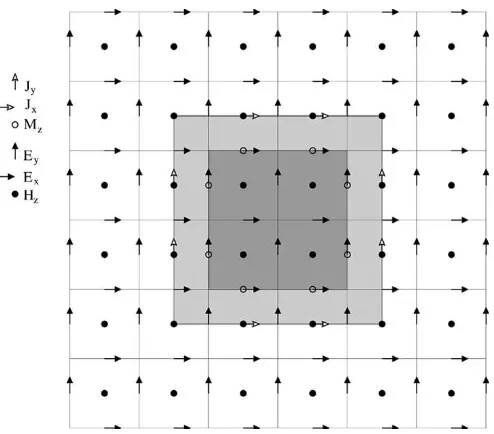
Fig. 1. Illustration of the concept of the Huygens’ box, shown in thexy-plane of a three-dimensional ADI-FDTD grid.
present are those requiring a separation between a total and a scattered field zone. For these problems, the equivalence principle is used to define on a closed Huygen’s surface a set of equivalent currents and so that the interior/exterior original sources of the problem can be removed. These currents are so defined to create the same fields as the original sources outside/inside, and null fields inside/outside (respectively). In order to implement the currents on the Huygen’s surface, the and components are interleaved in the Yee grid in a similar way to that of the and components, which results intwo
Huygen’s surfaces separated by a distance of half a cell. As an example, Fig. 1 shows the positions of , , , , and at the –plane. This method of implementing the equivalence principle in an FDTD computer code was first introduced in [12]; it does not require an averaging of the magnitudes involved.
In the first numerical experiment, we have placed on the sur-face of an empty Huygens’ box the currents necessary to create a 10-GHz plane wave of amplitude propa-gating inside the box along the –axis, and a null field outside. The cubic Huygen’s box spans 20 grid cells in each direction. A grid resolution of 60 cells/wavelength (
) is chosen for this experiment. We define the av-erage volumetric electric energy density at a point as follows:
(24)
144 IEEE ANTENNAS AND WIRELESS PROPAGATION LETTERS, VOL. 3, 2004
Fig. 2. Square root of the average electric energy density computed at a grid point outside the Huygens’ box, normalized to that of the incident plane wave as a function of the Courant number in the ADI-FDTD simulation.
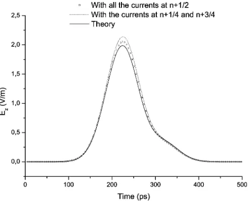
Fig. 3. Electric field computed at a point inside a Huygens’ box, generated by equivalent currents corresponding to a dipole placed outside the box.
with the time increment. We note that the increase in the error (a nonzero field outside the Huygen’s box) can be attributed in part to the intrinsic numerical dispersion error which also increases with the time increment.
The results of a second numerical experiment are shown in Fig. 3. Here, we plot the –component of the electric field gener-ated at a point inside a Huygens’ box by the equivalent currents corresponding to a dipole placed outside the box. The dipole is oriented along the –axis and is excited with a differentiated
Gaussian pulse. The simulation is conducted with a temporal sampling resolution of 21 time steps per period at the maximum frequency (defined as the decay point in the pulse spec-trum) and a spatial grid resolution of 60 cells per wavelength at that frequency, which corresponds to a Courant number of 4.9. Again the results obtained with the currents evaluated at in both subiterations are more accurate than those obtained with the currents evaluated at different discrete time values in the two subiterations.
V. CONCLUSION
Using a systematic approach to build the ADI–FDTD pro-cedure as a perturbation of the Crank–Nicolson scheme, we have obtained a new method of implementing current sources in ADI–FDTD. A theoretical analysis and numerical experiments demonstrate that this approach offers improved accuracy rela-tive to previously reported current source formulations.
REFERENCES
[1] T. Namiki, “A new FDTD algorithm based on alternating-direction implicit method,”IEEE Trans. Microwave Theory Tech., vol. 47, pp. 2003–2007, Oct. 1999.
[2] F. Zheng, Z. Chen, and J. Zhang, “A finite-difference time-domain method without the Courant stability conditions,” IEEE Microwave Guided Wave Lett., vol. 9, pp. 441–443, Nov. 1999.
[3] S. G. García, T. W. Lee, and S. C. Hagness, “On the accuracy of the ADI-FDTD method,”IEEE Antennas Wireless Propagat. Lett., vol. 1, pp. 31–34, 2002.
[4] T. Namiki, “Investigation of numerical errors of the two-dimensional ADI-FDTD method,”IEEE Trans. Microwave Theory Tech., vol. 48, pp. 1950–1956, Nov. 2000.
[5] A. Zhao, “Two special notes on the implementation of the uncondition-ally stable ADI-FDTD method,”Microwave Opt. Technol. Lett., vol. 33, pp. 273–277, May 2002.
[6] T.-W. Lee and S. C. Hagness, “Wave source conditions for the uncondi-tionally stable ADI-FDTD method,” inProc. IEEE Antennas and Prop-agation Society Int. Symp., vol. 4, Boston, MA, July 2001, pp. 142–145. [7] K. S. Yee, “Numerical solution of initial boundary value problems in-volving Maxwell’s equations in isotropic media,”IEEE Trans. Antennas Propagat., vol. 14, pp. 302–307, Mar. 1966.
[8] W. F. Ames, Numerical Methods for Partial Differential Equa-tions. New York: Academic, 1977.
[9] D. W. Peaceman and H. H. Rachford, Jr., “The numerical solution of parabolic and elliptic differential equations,”J. Soc. Ind. Appl. Math., vol. 3, pp. 28–41, 1955.
[10] J. Douglas, “On the numerical integration ofu +u = u by implicit methods,”J. Soc. Ind. Appl. Math., vol. 3, pp. 42–65, 1955.
[11] A. Taflove and S. Hagness,Computational Electrodynamics: The Finite-Difference Time-Domain Method, 2nd ed. Boston, MA: Artech House, 2000.
[12] D. E. Merewether, R. Fisher, and F. W. Smith, “On implementing a nu-meric Huygen’s source scheme in a finite difference program to illumi-nate scattering bodies,”IEEE Trans. Nucl. Sci., vol. 27, pp. 1829–1833, Dec. 1980.