Full Terms & Conditions of access and use can be found at
http://www.tandfonline.com/action/journalInformation?journalCode=ubes20
Download by: [Universitas Maritim Raja Ali Haji] Date: 12 January 2016, At: 00:16
Journal of Business & Economic Statistics
ISSN: 0735-0015 (Print) 1537-2707 (Online) Journal homepage: http://www.tandfonline.com/loi/ubes20
Structural Vector Autoregressions With
Nonnormal Residuals
Markku Lanne & Helmut Lütkepohl
To cite this article: Markku Lanne & Helmut Lütkepohl (2010) Structural Vector
Autoregressions With Nonnormal Residuals, Journal of Business & Economic Statistics, 28:1, 159-168, DOI: 10.1198/jbes.2009.06003
To link to this article: http://dx.doi.org/10.1198/jbes.2009.06003
Published online: 01 Jan 2012.
Submit your article to this journal
Article views: 211
Structural Vector Autoregressions With
Nonnormal Residuals
Markku L
ANNEDepartment of Economics, University of Helsinki, P.O. Box 17 (Arkadiankatu 7), FI-00014 Finland (markku.lanne@helsinki.fi)
Helmut L
ÜTKEPOHLDepartment of Economics, European University Institute, Via della Piazzola 43, I-50133 Firenze, Italy (helmut.luetkepohl@eui.eu)
In structural vector autoregressive (SVAR) modeling, sometimes the identifying restrictions are insuffi-cient for a unique specification of all shocks. In this paper it is pointed out that specific distributional assumptions can help in identifying the structural shocks. In particular, a mixture of normal distributions is considered as a possible model that can be used in this context. Our model setup enables us to test restrictions which are just-identifying in a standard SVAR framework. The results are illustrated using a U.S. macro data set and a system of U.S. and European interest rates.
KEY WORDS: Cointegration; Impulse responses; Mixed normal distribution; Vector autoregressive process; Vector error correction model.
1. INTRODUCTION
Structural vector autoregressive (SVAR) models are standard tools for empirical economic analysis. The basic underlying model is usually a vector autoregressive (VAR) or vector error correction (VEC) model in reduced form. If one wants to use these models for impulse response analysis, structural informa-tion is required to identify the relevant shocks and impulse re-sponses. Such information usually comes from economic the-ory or from structural and institutional knowledge related to a specific model setup or the variables involved. If some of the variables are integrated or cointegrated, long-run restric-tions may also be derived from the cointegration properties of the data. In many cases there is not enough information from such sources, however, to fully identify all shocks and impulse responses. In that situation different plausible restrictions are sometimes considered and the robustness of the main results with respect to uncertain identifying assumptions may be in-vestigated.
In this study it is argued that distributional assumptions can be helpful in identifying shocks of interest and in particular they may be substituted for missing identifying information from other sources. We use an idea put forward byLanne and Saikko-nen(2007) in the context of multivariate GARCH models and consider a mixture of normal distributions for the error terms of our basic model. In VAR analyses it is not uncommon that nonnormal residuals are found. Thus, it is plausible to specify more general distributions explicitly. A mixture of normal dis-tributions is useful, for instance, if the residual distribution has heavy tails and produces “outliers.” In that case one may think of the outliers as being generated by a different distribution than the remaining observations and identification of the shocks is obtained from heteroscedasticity across regimes. Thereby, our approach has some resemblance to that proposed byRigobon
(2003) and Rigobon and Sack(2003) for identifying shocks in SVAR models. These authors assume that there are regimes
with different covariance structures. However, they use the as-sumption of changes in the covariance at fixed points during the sampling period and use the associated heteroscedasticity for identification while in our setup the regimes are viewed as being generated stochastically. In fact, in our model setup the unconditional distribution of the residuals is homoscedas-tic. Generally, the class of mixed normal distributions is more flexible than the normal distributions and, hence, it may be use-ful whenever the class of normal distributions is too narrow.
In the following, conditions will be discussed which ensure identification of shocks if they have a mixture of two normal distributions. We will also discuss how this kind of identifi-cation can be combined with restrictions from other sources. Thereby it becomes possible to test restrictions which are just-identifying in the usual SVAR framework. For example, if coin-tegrated systems are considered, the number of shocks with exclusively transitory effects is often assumed to be identical to the number of cointegration relations and, accordingly, the number of shocks with permanent effects equals the number of common trends. In our framework such an assumption can be checked by testing the implied restrictions even if the shocks are not identified in a standard SVAR model. We will discuss tests for the number of transitory and permanent shocks in a coin-tegrated SVAR model and we will also consider tests of other restrictions which are just-identifying in the standard setup.
Two empirical examples will be presented to illustrate SVAR modeling with mixed normal residuals. The first one consid-ers the impact of fundamental shocks on real stock prices in the U.S. It is based on a system of stationary variables and primarily serves to illustrate some advantages of the mixed normal SVAR model relative to the standard approach. The second example considers a data set from Brüggemann and Lütkepohl(2005)
© 2010American Statistical Association Journal of Business & Economic Statistics January 2010, Vol. 28, No. 1 DOI:10.1198/jbes.2009.06003
159
consisting of two European and two U.S. interest rates which are cointegrated. We will be able to test some of the assump-tions of the previous analysis and find that they are not sup-ported in our modeling framework. As in the previous study, we find support for the view that U.S. monetary policy has a stronger impact on European interest rates than vice versa.
Our study is structured as follows. In the next section the general model setup is presented and identifying restrictions are discussed. Estimation of the models is considered in Section3
and the two examples are presented in Section4. Extensions and conclusions are provided in Section 5. A result related to mixture normal distributions is given in theAppendix.
2. THE MODEL SETUP
2.1 The Reduced Form
Consider the following n-dimensional reduced form VAR model of orderp,
A(L)yt=ut, (2.1) where A(L)=In−A1L− · · · −ApLp is a matrix polyno-mial in the lag operatorLwith(n×n)coefficient matricesAj (j=1, . . . ,p)andIndenotes the(n×n)identity matrix. The
n-dimensional error termut is assumed to be a mixture of two serially independent normal random vectors such that
ut=
e1t∼N(0,1) with probabilityγ,
e2t∼N(0,2) with probability 1−γ. (2.2) HereN(0,)denotes a multivariate normal distribution with zero mean and covariance matrix . The(n×n) covariance matrices1and2are assumed to be distinct and the mixture probabilityγ, 0< γ <1, is also a parameter of the model. If
1=2,uthas aN(0,1)distribution andγis not identified. Therefore we assume1=2. This assumption does not rule out that parts of1and2 are identical, in which case some components ofut may have normal distributions. In fact, it is enough that there is a single component inutwhich is not nor-mal. Notice also thatut has mean zero and covariance matrix
u=γ1+(1−γ )2, that is,ut∼(0, γ1+(1−γ )2). In (2.1) deterministic terms are neglected for simplicity. They can be added easily to the model without affecting the essential parts of the following discussion. We have dropped them from the model because they do not have a role in structural modeling and impulse response analysis.
2.2 Structural Restrictions for Levels VARs
The structural shocks, say εt, are usually defined such that they are zero mean uncorrelated random variables with unit variances, that is, εt ∼(0,In). In a so-called B model setup they are related to the reduced form errorsutbyut=Bεt (see Lütkepohl2005, chapter 9, for a detailed introductory account of these models). Clearly, E(utu′t)=u=BB′ andB is not
unique in general. Thus, to identify the structural shocks, re-strictions have to be imposed onB. Because the elements inB
represent the instantaneous effects of the shocks on the vari-ables, economic theory or institutional knowledge sometimes suggests zero restrictions forB. In other words, some shocks do not have an instantaneous impact on some of the variables.
A popular way to chooseBis to consider a triangular matrix which may be obtained from a Choleski decomposition ofu.
The shocks then have a recursive structure where for a lower triangular matrixBthe first shock can have an instantaneous impact on all the variables, whereas the second one may only influence the second to last variables instantaneously and so on. Although such a triangular orthogonalization of the resid-uals may occasionally be justified on theoretical grounds, it is sometimes chosen because no generally accepted theoretical constraints are available.
Another, by now quite popular, way to restrictB was pro-posed byBlanchard and Quah (1989). They argue that there may be reasons to assume that a specific shock may not have an accumulated long-run effect on a particular variable. In a stationary VAR model, the accumulated long-run effects of the shocks are given byA(1)−1B. Restricting one of the elements of this matrix to zero amounts to a restriction Rvec(B)=0
on B, where R=J(In⊗A(1)−1) and J is a suitable selec-tion matrix which selects those elements from vec(A(1)−1B)= (In⊗A(1)−1)vec(B)which are assumed to be zero (see Lütke-pohl2005, section 9.1.4, for details). We will consider this type of restriction in the first example in Section4.
Given our distributional assumption forut, there is another possibility to choose a unique matrix B. It is shown in Ap-pendixAthat a diagonal matrix=diag(ψ1, . . . , ψn),ψi>0 (i=1, . . . ,n) and a (n×n) matrix W exist such that 1=
WW′ and2=WW′ andW is unique apart from chang-ing all signs in a column, provided all ψi’s are distinct. In that case we can find a (locally) unique matrixBby choosing
B=W(γIn+(1−γ ))1/2. If the mixed normal distribution represents data from two different regimes such a choice ofB
amounts to assuming that shocks are orthogonal regardless of the regime they are coming from,N(0,1)orN(0,2), and, of course,εthas an identity covariance matrix. Local identifica-tion is all we can hope for in SVAR modeling because all signs in a column ofBcan always be reversed without changing the productBB′. In other words, it has to be decided whether one wants to consider positive or negative shocks.
Notice that identification is achieved by utilizing the spe-cific structure of the covariance matrix only. Such a structure is also obtained, of course, if any two distributions with mean zero and covariance matrices1and2are mixed. Assuming mixed normality is just a convenience which makes estimation straightforward while at the same time it allows for a very gen-eral and flexible class of distributions which can capture non-normal features observed in real data.
Clearly our identification of the shocks is a statistical one which is plausible because it ensures orthogonality of the shocks. It does not necessarily suggest an economic interpre-tation. In particular, it does not ensure that shocks can be asso-ciated with the variables of the system. For an economic inter-pretation the economic context has to be taken into account. For instance, in the first empirical example in Section4we investi-gate the impact of fundamental shocks on the stock market. In a simplified version of the model suppose that a system of two variables only is considered, wherey1andy2represent output growth and stock returns, respectively. A fundamental shock is one which has a permanent effect on output and possibly stock returns as well whereas a nonfundamental shock is character-ized by the property that it does not have a permanent effect on
Lanne and Lütkepohl: Structural Vector Autoregressions With Nonnormal Residuals 161
output. It may also have a permanent effect on stock returns, however. The standard approach is to assume that one of the two shocks in the system, say the second one, is nonfundamen-tal. Thereby one zero restriction is specified for the matrix of cumulative long-run responses,
Here the asterisks indicate unrestricted elements and the upper-right hand element is constrained to be zero. In this example the zero restriction on the matrixA(1)−1Bidentifies both shocks. In other words, it ensures that the matrixBsatisfyingBB′=u
is unique apart from possible changes in sign. Thus, in the stan-dard SVAR approach identification is achieved by the assump-tion that the two shocks are orthogonal and one of the shocks is nonfundamental. The latter assumption is made for identifica-tion purposes. It is not obvious that there is necessarily a non-fundamental shock in a bivariate system consisting of the two variables output growth and stock returns. Notice that, although there are nonfundamental shocks in a full economic system, it may not be possible to isolate them in a bivariate system of the simple type considered here. To avoid the assumption of the existence of a nonfundamental shock one may consider the sta-tistical properties of the data and use the approach based on the mixed normal residual distribution. For the present example it may be justified as follows.
In a system with financial variables nonnormal residuals are often considered. In fact, for higher frequency financial data, nonnormality due to conditional heteroscedasticity is often di-agnosed. If quarterly data are considered, as we will do in our first empirical example in Section4, it may be more plausible to suppose that the nonnormality is due to some outliers, that is, one may think of two regimes, one with a normal volatil-ity and one which has a larger volatilvolatil-ity and, hence, produces occasional outliers. In fact, it was found that ARCH tests may confuse outliers with conditional heteroscedasticity (e.g., van Dijk, Franses, and Lucas1999). Thus, suppose that our system has a nonnormal residual distribution, where the nonnormal-ity is due to outliers. In this situation considering a mixture of two normal distributions as in (2.2) is plausible. Decom-posing1=WW′ and 2=WW′ as in Appendix Athe
2matrix may, for instance, be made up of=diag(1, ψ2) with a largeψ2(>1)because the outliers may occur primarily in the stock returns variable. The crucial property here is that the two diagonal elements of are distinct. In this setup iden-tification of the two shocks is obtained by the requirement that the shocks have identity covariance matrix and are orthogonal in both the normal and the outlier regimes which is ensured by choosingB=W(γI2+(1−γ ))1/2. This choice implies thatB−1uB−1′=I2,B−11B−1′=(γI2+(1−γ ))−1, and
B−1
2B−1′=(γI2+(1−γ ))−1. Thus, this choice ofB diagonalizesu,1, and2simultaneously and thereby pro-vides shocks which are orthogonal in both regimes.
ThisBmatrix may or may not fit together with the previous assumption of having one nonfundamental shock. Because the latter assumption is not needed for identification of the shocks in the present mixed normal setup, the zero restriction in (2.3) which specifies that the second shock is nonfundamental now becomes testable. In fact, a likelihood ratio (LR) test is an ob-vious choice in this case because we have made a distributional assumption. If the nonfundamentalness assumption turns out to
be in line with the data, the impact of the fundamental shock on stock returns can be checked as in the standard framework. However, it is also possible that both shocks are found to be fundamental in the sense that both have permanent effects on output. Given that orthogonality of the shocks is a widely ac-cepted assumption in SVAR analysis, one may not be prepared to sacrifice it. Hence, in this situation there may simply not be a nonfundamental shock in our system. Notice, however, that even in our setup where a mixed normal residual distribution is used, one can always decomposeusuch that orthogonality
of the shocks goes together with the long-run restriction. Struc-tural shocks constructed in this way would not be orthogonal in both regimes, however. In summary, in this example the main difference between the standard SVAR approach and our setup is that the former assumes overall orthogonality of the shocks and that one of them is nonfundamental whereas our approach identifies the shocks by assuming that they are orthogonal in both regimes.
Of course, our framework is more general than reflected in this simple example. It can be used whenever the residual distri-bution is nonnormal. The interpretation of having two regimes with different variances may not be plausible in all cases and, hence, there may be good reasons for giving preference to some economically justified restrictions for identifying the structural shocks. If no such restrictions exist, it may still make more sense to use our statistical identification of the shocks rather than considering some arbitrary recursiveness assumption.
Our setup can also be combined with the standard SVAR ap-proach in those cases, where only some but not all of the shocks are identified by restrictions from the economic context. Sup-pose thatmshocks are identified by directly restrictingBand assume without loss of generality that they are placed in the last
mpositions ofεt. Then, for just-identification of all shocks, in the decomposition 2=WW′ with =diag(ψ1, . . . , ψn) only the first n−m ψi’s have to be distinct. If some of the lastmψi’s are also distinct, the shocks are actually overidenti-fied. In that case restrictions can be tested as long as the shocks remain identified under the null hypothesis. Generally, if ut has a general mixed normal distribution with covariance ma-trixW(γIn+(1−γ ))W′, where all diagonal elements of are distinct, restrictions for the shocks from other sources can be tested.
Although we have just discussed the B model for ease of exposition, similar considerations apply for the more general so-calledAB-model ofAmisano and Giannini(1997) (see also Lütkepohl 2005, chapter 9). In that case the structural shocks are such thatut=A−1Bεt and identifying restrictions may be placed on bothAandB. In the previous discussion,Bjust has to be replaced byA−1Bto cover this more general case. 2.3 Models With Cointegrated Variables
If some of the variables areI(1), then a VEC version of the VAR process is often more useful in structural analysis because it separates the long-run from the short-run movements of the variables and therefore makes it easy to impose restrictions on the long-run behavior of some or all of the shocks. We use the setup proposed byKing et al.(1991). The VEC representation of the model (2.1) is (see Lütkepohl2005, section 6.3)
yt=αβ′yt−1+Ŵ1yt−1+ · · · +Ŵp−1yt−p+1+ut, (2.4)
where=1−Lis the differencing operator,β is an(n×r) cointegration matrix with cointegrating rankr<n,αis an(n×
r)loading matrix for the cointegration relations, that is,αβ′yt−1 is the error correction term with long-run relationsβ′yt, and the
Ŵj’s are(n×n)short-run coefficient matrices. The parameters in (2.4) and (2.1) are related by the operator equationA(L)=
In−αβ′L−Ŵ1L− · · · −Ŵp−1Lp−1.
In this setup the long-run effects of the structural shocks can be shown to be Bin theB-model, where=β⊥[α′⊥(In−
p−1
i=1Ŵi)β⊥]−1α′⊥. The symbolsα⊥andβ⊥denote orthogo-nal complements ofαandβ, respectively (see Johansen1995). Becauseα andβ both have rank r, the matrix and, hence,
Bmust have rankn−r. It follows that at mostrof the shocks may have transitory effects only and, hence, they are associated with zero columns in the long-run matrixB. Such shocks will be called transitory in the following whereas shocks which have a permanent effect on at least one variable (at least one nonzero element in the associated column of the B matrix) will be called permanent. If a shock is known to be transitory, zero re-strictions on the long-run matrix may be imposed and used for identifying the structural shocks. In some cases this may even result in just-identified shocks. If there is more than one tran-sitory shock or more than one permanent shock, additional re-strictions will be needed, however. If they are not available from other sources, the mixture normal distribution may be helpful again.
Suppose that there are r transitory shocks, εtt, and n−r
permanent shocks, εpt, and they are arranged such that ε′t= (εpt′,εtt′). Hence,B= [ n×(n−r):0n×r], where n×(n−r)is an (n×(n−r))matrix. Furthermore, suppose that there are no other zero restrictions available forBandB. Then it is easy to see that the shocks are identified if ut has a mixed normal distribution as in (2.2) with covariance matrices 1=WW′ and2=WW′, where theψ1, . . . , ψn−rare distinct and also ψn−r+1, . . . , ψnare distinct.
Notice that in a VEC model with cointegration rankr<n
all structural shocks can in principle be permanent shocks ac-cording to our terminology because the matrix B may not have zero columns even if it has reduced rank. Treating ex-actlyr shocks as transitory is an assumption which is ideally not based purely on the cointegrating rank. Ifuthas a fully gen-eral mixed normal distribution as in (2.2), the zero constraints on B are, in fact, overidentifying restrictions which can be tested, for example, by LR tests. Hence, in this case we can test for the number of transitory and permanent shocks. Denoting the number of transitory shocks by r∗, we can, for example, test the null hypothesisH0:r∗=ror, equivalently,H0:B= [ n×(n−r):0n×r]against the alternative hypothesisH1:r∗<r, that is, Bis unrestricted. Alternatively, we may test against
H1:r∗=r−1, that is,B= [ n×(n−r+1):0n×(r−1)]. We can also test a sequence of null hypotheses H0:r∗=r,H0:r∗=
r−1, . . . ,H0:r∗ =1 to determine the number of transitory shocks. The testing sequence stops and the number of transi-tory shocks is chosen accordingly if one of the null hypotheses cannot be rejected.
3. ESTIMATION
Because a specific distribution for the reduced form error term is used, maximum likelihood (ML) is a plausible
estima-tion method. The error termuthas density φu(ut)=γ (2π )−n/2det(1)−1/2exp−12u′t diag(ψ1, . . . , ψn), as before. Using this parameterization and neglecting the constant terms, the conditional distribution ofyt givenYt−1=(yt−1,yt−2, . . . ,y−p+1)has a density (apart from Collecting all the parameters in the vectorϑ, the essential log-likelihood function can be written as
lT(ϑ)= T
t=1
logf(yt|Yt−1).
As discussed earlier, the parameters inWare identified if the ψi’s are all distinct. IfWand, hence,ϑis identified,lT(ϑ)can be maximized with standard nonlinear optimization algorithms. If such algorithms have convergence problems, this may be an indication of a lack of identification. Alternatively, we could use the parameterizations in terms of1and2and estimate these parameters first and then decompose the estimates to ob-tain estimates ofWand.
For stationary processes we can appeal to standard ML the-ory and conclude that for identifiedϑ the estimators have the usual limiting properties, that is, they are consistent and asymp-totically normal. Restrictions can be tested by LR tests using the usualχ2limiting distributions if the model is identified under both the null and alternative hypotheses.
For VEC models, if the cointegration relations are not known from subject matter theory, they may be estimated in a first step by theJohansen(1995) reduced rank regression which is equiv-alent to ML for a Gaussian model but is just a quasi-ML proce-dure under the present mixture normal assumption. In a second step we may then condition on the estimated cointegration rela-tions and maximize the log-likelihood with respect to the other parameters.
Generally ML estimation may be a computational challenge if a high-dimensional system with large lag orderp is consid-ered. In that case, using an EM algorithm for maximizing the likelihood function may be helpful (see Hamilton 1994, sec-tion 22.3, for a detailed derivasec-tion of a special case). Alterna-tively, one may consider estimation algorithms which do not result in full ML estimates. For example, two-step algorithms may be used which estimate the VAR coefficients in a first step by least squares methods and then estimate the parameters of the mixed normal distribution from the first-stage residuals. For our purposes the aforementioned ML methods are sufficient. Therefore, we do not elaborate on alternative methods at this stage. We believe, however, that alternative estimation methods may be a fruitful area of future research.
Lanne and Lütkepohl: Structural Vector Autoregressions With Nonnormal Residuals 163
4. EXAMPLES
In this section the previously discussed results will be illus-trated with two empirical examples. The first one uses a small system of U.S. macro variables fromBinswanger(2004). The second example considers a system of four interest rate series from the U.S. and Europe. It uses data which were analyzed earlier byBrüggemann and Lütkepohl(2005).
4.1 U.S. Model
There has been some discussion in the literature regarding the impact of fundamental shocks on the stock market. For ex-ample, in an SVAR analysisRapach (2001) finds that macro shocks have an important effect on real stock prices whereas
Binswanger(2004) concludes from his analysis that real activ-ity shocks explain only a small fraction of the real stock price variability in the U.S. for a period starting in the early 1980s. Clearly, in these studies the specification of the shocks is of cru-cial importance. We use a set of variables which was also ana-lyzed byBinswanger(2004). More precisely, we use quarterly U.S. data for the period 1983Q1–2006Q3 for the three variables log real gross domestic product (gdpt), the 3-month U.S. Trea-sury bill rate (rt), and log real stock prices (spt). Precise data sources are given in AppendixB. Note thatBinswanger(2004) included only data up to 2002 in his study. His objective was to assess the importance of fundamental shocks for stock price movements. Although there is no precise definition of funda-mental shocks, the idea is that these are shocks which may have a long-term impact on economic growth and the interest rate.
Binswanger(2004) found that all variables areI(1)and not cointegrated. Thus, he used a VAR model in first differences with lag orderp=4 foryt=(gdpt, rt, spt)′. We have con-firmed these specifications for our extended sample period us-ing standard unit root and cointegration tests as well as model specification criteria.Binswanger(2004) assumes that there is just one nonfundamental shock which may have a long-term impact on stock prices,spt, but not ongdptandrt. He identifies the three structural shocks by assuming that
A(1)−1B=
where again an asterisk denotes an unrestricted element so that the matrix is lower-triangular. The two zeros in the last col-umn are dictated by the assumption that the last shock is the nonfundamental one without long-term impact ongdptandrt. On the other hand, there is little justification for the additional zero restriction in the second column. It is imposed because it is required for identifying the shocks in the classical SVAR
framework and is to some extent arbitrary. Therefore identify-ing the shocks without such a restriction is desirable. Also, it may be useful to check whether the existence of a nonfunda-mental shock is a reasonable assumption for the system under consideration.
For the present system, standard Jarque–Bera nonnormality tests reject the normality hypothesis for the residuals. Hence, there is some support for using a nonnormal residual distrib-ution. In fact, the nonnormality may be due to a number of large residuals (outliers) which may be captured by a mixed normal distribution. Notice also that in the present setup, where the residuals are assumed to be from a mixed normal distri-bution which includes the normal distridistri-bution if1=2, the nonnormality test may be viewed as a test of the null hypothesis
H0:1=2. This hypothesis is clearly rejected by the Jarque– Bera test. Therefore, we have estimated the model with mixed normal residuals under the assumption that1=2. (All com-putations were done with GAUSS programs. The BHHH pro-cedure as implemented in the CML library of GAUSS was used for computing the ML estimates.) We have also estimated the model with the structural restrictions specified in (4.1) and without the zero restriction in the second column so that
A(1)−1B=
Some results are presented in Table1.
Since the restrictions in (4.1) and (4.2) are overidentifying if the ψi’s are distinct, we have first checked whether the lat-ter condition is satisfied. From the results in Table1 it is not obvious that all threeψi’s are really distinct in the unrestricted model [Model (1) in Table 1] because the estimated standard errors are relatively large. We have therefore performed Wald tests of the null hypotheses listed in Table 2. Since the esti-mators have the usual normal limiting distributions under our assumptions, the Wald tests have asymptotic χ2-distributions and the resultingp-values are given in Table2. Notice that the ψi’s are identified even if they are identical whereas the ma-trixWwill then not be unique. Thus, we can test equality of theψi’s. It turns out that we cannot reject equality of all three ψi’s in the unrestricted model. However, potentially more pow-erful pairwise comparisons reveal that two of the threeψi’s may be different. More precisely, the hypothesesH0:ψ1=ψ2and
H0:ψ1=ψ3can be rejected at the 10% level in the unrestricted model. In contrast,p-values of at least 10% are obtained for all tests based on the model where the restrictions (4.1) are im-posed [Model (2) in Table1]. On the other hand, a Wald test of
H0:ψ1=ψ2has ap-value of less than 10% if the restrictions in (4.2) are imposed [see Model (3) in Table1]. Thus, if the restric-tions (4.2) are imposed, there is some evidence thatψ1=ψ2.
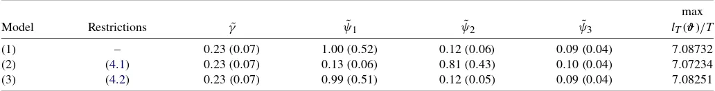
Table 1. Estimation results for U.S. SVAR model with lag orderp=4 and intercept term (sample period: 1984Q2–2006Q3)
max
Model Restrictions γ˜ ψ˜1 ψ˜2 ψ˜3 lT(ϑ)/T
(1) – 0.23(0.07) 1.00(0.52) 0.12(0.06) 0.09(0.04) 7.08732
(2) (4.1) 0.23(0.07) 0.13(0.06) 0.81(0.43) 0.10(0.04) 7.07234
(3) (4.2) 0.23(0.07) 0.99(0.51) 0.12(0.05) 0.09(0.04) 7.08251
NOTE: Standard errors in parentheses obtained from the inverse Hessian of the log-likelihood function.
Table 2. p-values of Wald tests for equality ofψi’s
This suggests that in the latter model the first two (fundamen-tal) shocks can be identified via the distributional assumption whereas the third shock is identified via economic reasoning.
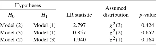
Assuming that the shocks in the model with restrictions (4.2) are in fact identified, the additional restriction in (4.1) is overi-dentifying and can be tested. The LR statistic and its associ-ated p-value are given in Table 3 [see H0: Model (2) versus
H1: Model (3)]. The latter quantity is 0.164 and, hence, we can-not reject the restriction even at a 10% level of significance. Thus, with our approach we end up with the same restrictions that were imposed byBinswanger(2004). The advantage of our approach is, however, that we have at least statistical support for imposing the additional restriction.
Although our tests in Table2suggest that theψi’s may not all be distinct, for illustrative purposes we also present thep-values of the likelihood ratio tests of the zero restrictions in (4.1) and (4.2) in Table3. Theχ2-distributions underlying thep-values are determined under the problematic assumption that theψi’s are all distinct and, hence, the structural shocks are identified via the mixed normal distribution. Under this assumption the restrictions cannot be rejected at usual significance levels (e.g., at 10%) which is in line with our previous result. If some of theψi’s are in fact identical, then the asymptotic distributions of the LR tests in Table 3may still be χ2 but they will have fewer degrees of freedom because some of the restrictions in (4.1) and/or (4.2) may not be overidentifying. In that case the actual asymptoticp-values would be smaller than the ones pre-sented in Table3. Given the magnitudes of the test values, it is not likely that a rejection were possible if the true degrees of freedom were known, however.
4.2 U.S. and European Interest Rates
Brüggemann and Lütkepohl(2005) considered euro area and U.S. short-term and long-term interest rates to investigate the relation between European and U.S. monetary policy. They found support for the hypothesis that European monetary policy responds to U.S. monetary policy whereas the reverse direction is not apparent from the data. They admit, however, that their analysis is partly based on arbitrary identification restrictions.
Table 3. LR tests based on results from Table1
Hypotheses
Hence, it is of interest to check whether the framework devel-oped in the present paper can be used to overcome the arbitrari-ness.
In a preliminary analysisBrüggemann and Lütkepohl(2005) concluded that both the expectations hypothesis of the term structure and the uncovered interest rate parity are supported. More precisely, they analyzed four monthly interest rate series for the period 1985M1–2004M12. The series are a euro area three-month money market ratertEU, a euro area 10-year bond rate REUt , a U.S. three-month money market rate rUSt , and a U.S. 10-year bond rateRUSt . Details on the data construction and their sources are given in AppendixB.Brüggemann and Lütkepohl(2005) found that all four variables areI(1)whereas the two spreadsRUSt −rUSt andREUt −rtEU as well as the two paritiesRUSt −REUt and rtUS−rEUt are stationary and, hence, there are three linearly independent cointegration relations in the system of four series.
Therefore,Brüggemann and Lütkepohl(2005) used a VEC model for yt =(RUSt ,rtUS,REUt ,rEUt )′ with a constant term, three lags ofyt, and a cointegrating rank of r=3 to inves-tigate the impact of monetary shocks in the U.S. and in Eu-rope. Because the cointegrating rank is r=3 they restricted three shocks to have transitory effects only. Thereby they iden-tified the permanent shock. It is not obvious why there should be three transitory shocks, however. The fact that there are three cointegration relations implies that there can be at most three transitory shocks. Of course, there could be fewer such shocks. Moreover, there is no well-accepted theory that suggests how to identify the transitory shocks. Because, based on standard Jarque–Bera tests, there is some evidence that the model resid-uals are nonnormal, using a more general distribution is plausi-ble.
We have estimated different models with mixed normal resid-uals and present some results in Table4, where the number of transitory shocks (i.e., the number of zero columns inB) is denoted byr∗. Clearly, theψ˜i’s are quite different in all mod-els. We have again tested equality of all pairs of ψi’s in the unrestricted model [Model (1) in Table4] using Wald tests and found that onlyH0:ψ3=ψ4cannot be rejected at the 5% level of significance. If there are indeed three differentψi’s, models with one, two, or three transitory shocks may still be identified. Based on the results in Table 4 we can test for the num-ber of transitory shocks as explained in Section2.3. The rel-evant results are given in Table5. Both tests,H0:r∗=3 versus
H1:r∗<3 and H0:r∗=3 versusH1:r∗=2 have very small
p-values and clearly reject at common significance levels, for example, at the 1% level. Note that if only threeψi’s are dif-ferent, the number of degrees of freedom may be lower than three. Hence, rejection of the null hypothesis would be possi-ble at an even smaller significance level. In other words, three transitory shocks are clearly rejected. Testing a model with only two transitory shocks, the result is more favorable. Both alter-native tests havep-values greater than 10% and, hence, using that significance level, indicate compatibility of two transitory shocks with the data in our setup. Clearly this result means that the model used by Brüggemann and Lütkepohl(2005) is not supported by the data in our setup and, hence, confirms the arbi-trariness of their identifying assumptions. The question is, how-ever, whether our approach allows us to go further and consider
Lanne and Lütkepohl: Structural Vector Autoregressions With Nonnormal Residuals 165
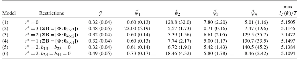
Table 4. Estimation results for interest rate VEC model with cointegrating rankr=3, three lagged differences and unrestricted intercept term (sample period: 1985M1–2004M12)
max
NOTE: Standard errors in parentheses obtained from the inverse Hessian of the log-likelihood function.
the relation between U.S. and European monetary policy. This issue will be considered in the following.
If one accepts that there are two transitory shocks and one places them in the last two positions of the vector of shocks, the discussion in Section2.3suggests that identification is ensured ifψ1=ψ2andψ3=ψ4. We have checkedH0:ψ1=ψ2 and
H0:ψ3=ψ4and obtainedp-values of 0.003 and 0.088, respec-tively. Thus, both null hypotheses are rejected at a 10% level. Therefore we assume in the following that a model with two transitory shocks [Model (3) in Table4] is identified.
To use our model to investigate the relation between U.S. and European monetary policy, we need to know more about the shocks in our model. We also give results of tests of interest for this purpose in the lower part of Table5. Because mone-tary policy shocks are sometimes thought of as being transi-tory (e.g., Evans and Marshall1998), the two transitory shocks in our system may represent monetary policy shocks in Eu-rope and the U.S., respectively. Without further restrictions they could, of course, both be mixtures of such shocks. One way to associate them uniquely with one of the two currency ar-eas would be to impose suitable restrictions. Therefore we used models with two transitory shocks and restricted the instanta-neous impact of one of them to be zero for the U.S. interest rates [Model (5) in Table4] and the other one has no instanta-neous impact on the European interest rates [Model (6) in Ta-ble4]. In other words, recalling the ordering of the variables in
yt=(RUSt ,rtUS,REUt ,rEUt )′, we impose the restrictions:
Table 5. LR tests based on results from Table4
Hypotheses
[Model (6) in Table4]. Restricting the first transitory shock (the third shock in theεtvector) to have no instantaneous effect on U.S. interest rates it cannot be the U.S. monetary policy shock and, hence, must be the European monetary shock if indeed each of the two transitory shocks represents one of the monetary policy shocks. Consequently, the third shock in our system is viewed as the European monetary policy shock and the fourth shock is regarded as U.S. monetary policy shock.
In Table 5 the corresponding restrictions are tested and it turns out that the constraints in (4.3) cannot be rejected at the 10% level of significance whereas the restrictions in (4.4) are clearly rejected at common significance levels (e.g., at the 1% level). Thus, the model with restrictions (4.3) is the preferred one and the first transitory shock can clearly be associated with European monetary policy. Moreover, European monetary pol-icy shocks do not seem to affect U.S. interest rates instanta-neously. On the other hand, U.S. monetary policy has an im-mediate impact on European interest rates because there is no transitory shock which affects only U.S. interest rates instanta-neously.
The finding that U.S. monetary policy may have an instan-taneous impact on European interest rates but not vice versa is in line with the conclusion of Brüggemann and Lütkepohl
(2005) that U.S. interest rates have a stronger impact on Eu-ropean monetary policy than vice versa. In their framework they could not formally test this result, however. Although also in our framework some assumptions are necessary (e.g., we assume that monetary policy shocks are transitory), statistical tests can carry us one step further in checking restrictions that are not overidentifying in the standard framework and, hence, cannot be tested in that setting.
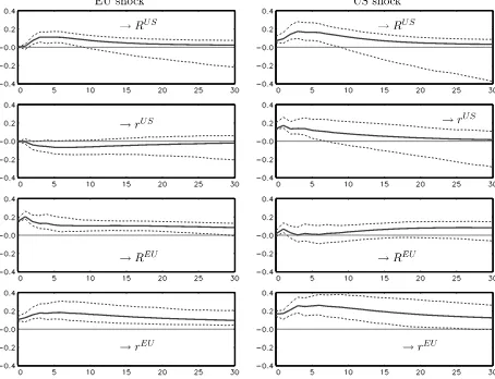
We have also computed the impulse responses for the two transitory shocks and show them in Figure 1 together with 95% bootstrap confidence intervals. These confidence intervals are based on 2,000 bootstrap replications using the method re-ferred to as Hall’s percentile method byBenkwitz, Lütkepohl, and Wolters(2001). They are presented here because they have a better theoretical foundation than the ones more commonly used in impulse response analysis. It turns out that a contrac-tionary EU shock leads to an increase in the U.S. long-term
Figure 1. Responses of interest rates to EU and U.S. monetary shocks based on Model (5) from Table4with 95% bootstrap confidence intervals (dashed lines) based on 2,000 bootstrap replications.
rate, although not instantaneously. There is no significant reac-tion of the U.S. short-term rate, however. In contrast, a contrac-tionary U.S. monetary shock has a significant instantaneous and longer lasting impact on the EU short-term rate and there is also a potentially significant impact on the EU long-term rate. Thus, overall the impulse responses are in line with the conclusion that U.S. monetary policy may be more important for Europe than vice versa. Thus, the conclusions drawn by Brüggemann and Lütkepohl (2005) based on a model with arbitrary iden-tifying restrictions can be confirmed in our framework which extracts identification restrictions from the statistical properties of the data.
5. CONCLUSIONS AND EXTENSIONS
In this paper we have used distributional assumptions for the residuals of a VAR model to identify some or all shocks to be used for an impulse response analysis or forecast error variance decomposition. Specifically we have used a mixture of two nor-mal distributions to obtain fully identified shocks. We have also shown how such nonnormal error distributions can be combined with restrictions from other sources to identify the shocks and impulse responses. For example, they can be combined with re-strictions derived from the cointegration properties of a system
of variables. Two empirical examples have been used to illus-trate the virtue of the approach for applied work.
Although in practice it will be easy to justify nonnormal distributions for many econometric models, our approach has some limitations that deserve further consideration in future work. First of all, we have considered mixtures of two zero mean normal distributions only. This may be reasonable if two different regimes are a plausible assumption for the sample pe-riod. Sometimes it may be more natural to allow for more than two regimes, however, and, hence, mix more than two normal distributions. Second, although we have argued that a mixture normal distribution is often a plausible extension of the usual normal distribution, there may be appealing alternative distrib-utions which are worth considering in this context. For exam-ple,Siegfried(2002) argues that monetary policy shocks may be leptokurtic and he considers a logistic distribution. He also presents an algorithm for estimating independent rather than just uncorrelated shocks. Generally, the potential of other dis-tributions for identifying the shocks in a structural VAR model may be worth investigating. Third, if one thinks of the mix-ture distribution as two distributions associated with two states of an economic system it may be plausible to make the state in a particular period dependent on the past states. For exam-ple, the states may be generated by a Markov chain whereas in our model the states are generated by an i.i.d. process. Us-ing a Markov chain for the process that generates the states in
Lanne and Lütkepohl: Structural Vector Autoregressions With Nonnormal Residuals 167
our setup amounts to considering a Markov regime switching model with changing residual covariance. Univariate models of this type were pioneered byHamilton(1989) and multivariate versions may be worth considering in the present context. Fi-nally, for the structural analysis a reduced form model has to be found which describes the data generation process well. Spec-ification and inference procedures which account for residuals with mixed normal and other nonnormal distributions may be worth exploring. Moreover, given the large number of parame-ters in full VAR models, ML estimation may be a computational challenge in some cases and it may be worth considering other estimation methods. We leave these issues for future research.
APPENDIX A: A MATHEMATICAL RESULT
In this appendix we present a proposition which is useful in dealing with the mixture normal distribution.
Proposition 1. Letube a mixture of two normal random vec-tors such that ance matrices with 1=2. Then there exist a nonsingular (n×n)matrixWand a diagonal matrix=diag(ψ1, . . . , ψn) with positive diagonal elements such that1=WW′and2=
WW′. The matrixWis unique up to reversal of all signs in a column if allψj’s are mutually different.
Proof. Because1and2are both symmetric positive def-inite, the existence of matricesW and=diag(ψ1, . . . , ψn) as in the proposition is a well-known matrix result [see Horn and Johnson 1985, 7.6.5 corollary, or Lütkepohl 1996, sec-tion 9.12.3 (4)]. Thus, it remains to show the uniqueness ofW
(apart from multiplication of its columns by−1) if allψi’s are distinct.
Suppose there exists a nonsingular matrix Q such that
1=WQQ′W′ and2=WQQ′W′. Then pre- and post-multiplying1byW−1andW′−1, respectively, shows thatQ must be an orthogonal matrix. Moreover,
=W−12W′−1=W−1WQQ′W′W′−1=QQ′, or, equivalently,Q=Q. Denoting theijth element ofQby
qij, the last matrix equality means thatψiqij=ψjqijand, hence,
qij=0 fori=jbecauseψi=ψj. Consequently,Qmust be a diagonal matrix with±1 on the diagonal because the diagonal elements of a diagonal matrix are its eigenvalues and the eigen-values of an orthogonal matrix are all±1.
APPENDIX B: DATA SOURCES
Quarterly U.S. data for the period 1983Q1–2006Q3 from the following sources are used for the example of Section4.1:
Interest rate: three-month U.S. Treasury Bill Secondary Market Rate take from FRED II (Series ID: TB3MS), the quarterly data are obtained as the values for the last month of each quarter.
Stock prices: Standard & Poor 500 Composite-price index taken from Datastream (Code: S&PCOMP); the real prices are
computed by using the U.S. Consumer Price Index (2000= 100) taken from Datastream (Code: USQ64...F).
GDP: U.S. real GDP at 2000 prices from Datastream (Code: USOCFGDPD).
The data used in the example of Section 4.2are the same ones used byBrüggemann and Lütkepohl(2005). In the follow-ing we reproduce the data sources given in that article. Monthly data for the period 1985M1–2004M12 are used. Euro area inter-est rate series correspond to German interinter-est rates for the period 1985M1–1998M12 and to euro area interest rates for the period 1999M1–2004M12. Monthly values are averages over all busi-ness days. The data are taken from the sources listed below:
U.S. long-term interest rate (RUS): 10-year T-Bill rate taken from FRED II database. Series ID: GS10.
U.S. short-term interest rate(rUS): 3-month money market rate taken from FRED II database. Series ID: CD3M.
Euro area long-term interest rate (REU): 1985M1–1998M12: 10-year government bond rate (Umlaufsrendite) taken from
Deutsche Bundesbank database. Series ID: WU0004. 1999M1–2004M12: 10-year euro area government bench-mark bond yield. Source: ECB monthly bulletin, T04.07_c5.
Euro area short-term interest rate(rEU): 1985M1–1998M12: 3-month money market rate taken from Deutsche Bun-desbank database. Series ID: SU0107. 1999M1–2004M12: 3-month money market rate (EURIBOR). Source: ECB monthly bulletin, T04.06_c3.
ACKNOWLEDGMENTS
The authors thank Jörg Breitung, Hashem Pesaran, Morten Ravn, Pentti Saikkonen, Ralf Brüggemann, two anonymous ref-erees, the editor Serena Ng, and participants of several work-shops and conferences for helpful comments on earlier versions of the paper. The first author acknowledges financial support from the Yrjö Jahnsson Foundation. Much of this research was done while he was a Jean Monnet Fellow in the Economics De-partment of the European University Institute.
[Received June 2006. Revised April 2008.]
REFERENCES
Amisano, G., and Giannini, C. (1997),Topics in Structural VAR Econometrics (2nd ed.), Berlin: Springer. [161]
Benkwitz, A., Lütkepohl, H., and Wolters, J. (2001), “Comparison of Boot-strap Confidence Intervals for Impulse Responses of German Monetary Systems,”Macroeconomic Dynamics, 5, 81–100. [165]
Binswanger, M. (2004), “How Do Stock Prices Respond to Fundamental Shocks?”Finance Research Letters, 1, 90–99. [163,164]
Blanchard, O., and Quah, D. (1989), “The Dynamic Effects of Aggregate De-mand and Supply Disturbances,”American Economic Review, 79, 655–673. [160]
Brüggemann, R., and Lütkepohl, H. (2005), “Uncovered Interest Rate Parity and the Expectations Hypothesis of the Term Structure: Empirical Results for the U.S. and Europe,”Applied Economics Quarterly, 51, 143–154. [159, 163-167]
Evans, C. L., and Marshall, D. A. (1998), “Monetary Policy and the Term Struc-ture of Nominal Interest Rates: Evidence and Theory,”Carnegie-Rochester Conference Series on Public Policy, 49, 53–111. [165]
Hamilton, J. D. (1989), “A New Approach to the Economic Analysis of Nonsta-tionary Time Series and the Business Cycle,”Econometrica, 57, 357–384. [167]
(1994), Time Series Analysis, Princeton, NJ: Princeton University Press. [162]
Horn, R. A., and Johnson, C. R. (1985),Matrix Analysis, Cambridge: Cam-bridge University Press. [167]
Johansen, S. (1995),Likelihood-Based Inference in Cointegrated Vector Au-toregressive Models, Oxford: Oxford University Press. [162]
King, R. G., Plosser, C. I., Stock, J. H., and Watson, M. W. (1991), “Stochastic Trends and Economic Fluctuations,”American Economic Review, 81, 819– 840. [161]
Lanne, M., and Saikkonen, P. (2007), “A Multivariate Generalized Orthogonal Factor GARCH Model,”Journal of Business & Economic Statistics, 25, 61–75. [159]
Lütkepohl, H. (1996),Handbook of Matrices, Chichester: Wiley. [167]
(2005),New Introduction to Multiple Time Series Analysis, Berlin: Springer-Verlag. [160,161]
Rapach, D. E. (2001), “Macro Shocks and Real Stock Prices,”Journal of Eco-nomics and Business, 53, 5–26. [163]
Rigobon, R. (2003), “Identification Through Heteroskedasticity,”Review of Economics and Statistics, 85, 777–792. [159]
Rigobon, R., and Sack, B. (2003), “Measuring the Reaction of Monetary Policy to the Stock Market,”Quarterly Journal of Economics, 118, 639–669. [159] Siegfried, N. A. (2002), “An Information-Theoretic Extension to Structural
VAR Modelling,” discussion paper, Hamburg University. [166]
van Dijk, D., Franses, P. H., and Lucas, A. (1999), “Testing for ARCH in the Presence of Additive Outliers,”Journal of Applied Econometrics, 14, 539– 562. [161]