Full Terms & Conditions of access and use can be found at
http://www.tandfonline.com/action/journalInformation?journalCode=ubes20
Download by: [Universitas Maritim Raja Ali Haji] Date: 12 January 2016, At: 23:56
Journal of Business & Economic Statistics
ISSN: 0735-0015 (Print) 1537-2707 (Online) Journal homepage: http://www.tandfonline.com/loi/ubes20
Do Panels Help Solve the Purchasing Power Parity
Puzzle?
Christian J Murray & David H Papell
To cite this article: Christian J Murray & David H Papell (2005) Do Panels Help Solve the
Purchasing Power Parity Puzzle?, Journal of Business & Economic Statistics, 23:4, 410-415, DOI: 10.1198/073500105000000072
To link to this article: http://dx.doi.org/10.1198/073500105000000072
Published online: 01 Jan 2012.
Submit your article to this journal
Article views: 74
View related articles
Do Panels Help Solve the Purchasing Power
Parity Puzzle?
Christian J. M
URRAYand David H. P
APELLDepartment of Economics, University of Houston, Houston, TX 77204 (cmurray@mail.uh.edu;dpapell@uh.edu)
Although Rogoff described the “remarkable consensus” of 3- to 5-year half-lives of purchasing power parity (PPP) deviations among studies using long-horizon data, recent works using panel methods with post-1973 data report shorter half-lives of 2 to 2.5 years. But these studies do not use appropriate tech-niques to measure persistence. We extend median-unbiased estimation methods to the panel context, cal-culate both point estimates and confidence intervals, and provide strong evidence confirming Rogoff’s original claim. Although panel regressions provide more information on the persistence of real exchange rate shocks than univariate regressions, they do not help solve the PPP puzzle.
KEY WORDS: Panel median-unbiased estimation; PPP puzzle; Real exchange rate persistence.
1. INTRODUCTION
Rogoff’s (1996) purchasing power parity (PPP) puzzle involves the difficulty of reconciling very high short-term volatility of real exchange rates with very slow rates of mean reversion. In a much-quoted phrase, Rogoff described the “remarkable consensus” of 3- to 5-year half-lives of PPP de-viations among various studies. The PPP puzzle has inspired a good deal of research, much of it directed at attempts to “solve” the PPP puzzle by reducing the half-lives.
The empirical work that Rogoff has cited in support of his 3- to 5-year consensus mostly comes from univariate studies with long-horizon data. More recent panel studies using quar-terly, post-Bretton Woods data with nominal exchange rates deflated by consumer price indexes and the U.S. dollar as the numeraire currency, including those of Wu (1996), Papell (1997, 2002), Fleissig and Strauss (2000), and Papell and Theodoridis (2001), found shorter half-lives of 2 to 2.5 years.
These shorter half-lives appear to be influencing perceptions of the magnitude of the PPP puzzle. Cheung, Chinn, and Fujii (2001) used 2 to 2.5 years to describe the results of the more recent studies. Engel and Morley (2001) used 2.5 to 5 years to describe the “typical” estimate of half-lives, followed by the quote from Rogoff (1996) that contains the 3- to 5-year con-sensus. Obstfeld (2001) wrote that “the best current estimates of real exchange rate persistence suggest that under floating nominal exchange rate regimes, the half-lives of real exchange rates shocks range from 2 to 4.5 years.” If the point estimate of half-lives of PPP deviations is 2.5 rather than 4 (the average of Rogoff’s 3 to 5) years, then it is much more likely that models with nominal rigidities (or future modifications of such models) will be able to “solve” the PPP puzzle.
In this article we argue that the evidence of shorter half-lives from panel methods applied to post-1973 data is misleading. The reason for this is straightforward. These studies typically use panel versions of augmented Dickey–Fuller (ADF) tests to investigate whether the null hypothesis of a unit root in real ex-change rates can be rejected. The least squares estimate of the parameter of interest, α, the sum of the autoregressive coeffi-cients, is significantly downward-biased in models that contain an intercept or an intercept and a time trend. The bias becomes more severe asαgets larger, which has particular relevance for the case of real exchange rates. Moreover, the half-life (the ex-pected number of years for a PPP deviation to decay by 50%) is a nonlinear function ofα, which accentuates the bias.
These issues were addressed in the univariate context for first-order autoregressive (AR) models by Andrews (1993), who showed how to calculate exactly median-unbiased esti-mates, as well as exact confidence intervals, for half-lives in Dickey–Fuller (DF) regressions. Andrews and Chen (1994) showed how to perform approximately median-unbiased es-timation in ADF regressions. Median-unbiased estimators have the desirable properties that their point estimates remain median-unbiased and the coverage probabilities of their confi-dence intervals are invariant under monotonic transformations. This is important because the least squares (LS) estimate of the half-life, ln(.5)/ln(αLS), is a monotonic transformation of the LS estimate,αLS. If we replace αLS with a median-unbiased estimate,αMU, then the half-life estimate will also be median-unbiased.
Murray and Papell (2002) used median-unbiased estimation methods with both annual long-horizon and quarterly post-1973 real exchange rate data. With long-horizon data, the median value of the point estimates of PPP deviations from the univari-ate regressions is 3.98 years, almost in the middle of Rogoff’s 3- to 5-year range. With post-1973 data, the median half-life is 3.07 years—near the bottom, but still within Rogoff’s consen-sus. The median bounds of the confidence intervals, especially with the post-1973 data, are much too wide to be informative, however.
Murray and Papell (2005) used these methods to reexam-ine the evidence of slow mean reversion for the long-horizon dollar–sterling real exchange rate found by Lothian and Taylor (1996). Using their specification, we show that they underesti-mated the half-lives of PPP deviations, and thus overestiunderesti-mated the speed of mean reversion. When we amend their specifica-tion to allow for serial correlaspecifica-tion, the speed of mean reversion falls even further. These results make resolution of the PPP puz-zle more problematic.
The purpose of this article is to extend median-unbiased es-timation methods to the panel context and to investigate the implications of these methods for the persistence of devia-tions from PPP. We first compute LS estimates of the half-life in panel ADF regressions. Using general-to-specific (GS)
© 2005 American Statistical Association Journal of Business & Economic Statistics October 2005, Vol. 23, No. 4 DOI 10.1198/073500105000000072 410
Murray and Papell: Panels and Purchasing Power Parity 411
lag selection, the point estimate of the half-life is 2.35 years, with bounds on the 95% bootstrap confidence interval (CI) of 1.29 and 2.22 years. With modified Akaike information crite-rion (MAIC) lag selection, the half-life estimate is 2.90 years, with a CI of [1.47,2.74]years. Although the point estimates seems reasonable, there is obviously something wrong when the upper bound of the 95% CI liesbelowthe point estimate. This failure of the bootstrap CI reflects the bias inherent in LS esti-mates of AR parameters, as well as an additional layer of bias, because the data-generating process in the bootstrap is based on a biased estimate.
We proceed to compute approximately median-unbiased esti-mates of half-lives in panel ADF regressions. Our median point estimate is 3.55 years, with bounds on the 95% CI of 2.48 and 4.09 years. We therefore conclude that panel methods applied to post-1973 data do not solve the PPP puzzle. Both the point estimates and the CIs are consistent with Rogoff’s 3- to 5-year consensus.
2. PERSISTENCE OF PURCHASING POWER
PARITY DEVIATIONS
PPP is the hypothesis that after a disturbance, the real ex-change rate reverts in the long run to a constant mean. We con-sider real exchange rates with the U.S. dollar as the numeraire currency, which are calculated as
q=e+p∗−p, (1)
whereqis the logarithm of the real exchange rate,eis the log-arithm of the nominal (dollar) exchange rate,pis the logarithm of the domestic consumer price index (CPI), andp∗is the loga-rithm of the U.S. CPI.
The DF model regresses the real exchange rate on a constant and its lagged level,
qt=c+αqt−1+ut. (2)
The null hypothesis of a unit root is rejected in favor of long-run PPP ifαis significantly less than unity. A time trend is not in-cluded in (2), because such an inclusion would be theoretically inconsistent with long-run PPP.
The ADF regression addskfirst differences of the real ex-change rate to (2) to allow for serial correlation,
qt=c+αqt−1+ k
j=1
ψjqt−j+ut. (3) Again, the unit root null is rejected in favor of long-run PPP if
αis significantly less than 1.
A panel extension of the DF regression that allows for het-erogeneous intercepts would involve estimating the equations
qit=ci+αqi,t−1+uit, (4) where the subscript i indexes the country and ci denotes the country-specific intercept. Alternatively, a panel extension of the ADF regression model that allows for a heterogeneous in-tercept, as well as serially and contemporaneously correlated errors, is written as
We follow Levin, Lin, and Chu (2002) and restrict the value ofα
to be equal for every country in the panel. The null hypothesis is that all of the series contain a unit root, and the alternative is that they are all stationary. This is in contrast with panel unit root tests, (e.g., Im, Pesaran, and Shin 2003), which allowαto vary across countries. In that case the null hypothesis is that all of the series contain a unit root and the alternative is that at least one of the series is stationary.
To allow for contemporaneous correlation of the errors, (4) and (5) are estimated using feasible generalized least squares (GLS) (seemingly unrelated regressions), withα equat-ed across countries. Abuaf and Jorion (1990) usequat-ed (4) for long-horizon annual data and set the value of k to 12 in (5) for post-1973 monthly data. Papell (1997) used heterogeneous val-ues for k and took them from the results of univariate ADF regressions using the GS criteria.
Our concern in this article is to calculate point estimates and confidence intervals of the speed of adjustment to PPP in the panel model, rather than to focus on the statistical question of whether or not the hypothesis of unit roots in real exchange rates can be rejected. The most commonly used measure of persistence is the half-life (the expected number of years for a PPP deviation to decay by 50%), calculated by ln(.5)/ln(α). In the univariate DF regression,αis a complete scalar measure of persistence. In the more general ADF regression, it is prefer-able to calculate the half-life from the impulse response func-tion, because ln(.5)/ln(α)assumes a monotonic rate of decay, which does not necessarily occur in higher-order AR models. In the panel ADF model, with or without serial correlation, the only way to calculate the half-life is from α, because the lag lengths (ki) and the serial correlation coefficients (ψij)in (5) vary across countries.
As described earlier, we restrict the value ofα, and thus the half-lives, to be equal for every country in the panel. To lend credence to our homogeneity restriction, we conducted Wald tests for the null hypothesis thatαi=α, assuming that the panel is stationary. For both methods of lag selection that we consider, we fail to reject the null hypothesis and proceed under the as-sumption that homogeneity is reasonable for this sample. Imbs, Mumtaz, Ravn, and Rey (2005) argued that cross-sectional ag-gregation can impart an upward bias to half-life estimates. But the estimated bias in their article, is due entirely to heterogene-ity of convergence rates among the sectors that make up na-tional price indexes, not to heterogeneity of convergence rates among the countries that make up their panels. Choi, Mark, and Sul (2004) failed to reject the homogeneity hypothesis for α
with the same panel of real exchange rates as ours, but in an AR(1)context with annual data from 1948 to 1998, and con-cluded that cross-country heterogeneity inαdoes not constitute a significant source of bias.
The problem with these half-life calculations is that the LS estimates ofαare significantly downward-biased for the vari-ants of the models that contain an intercept and have a value of α fairly close to unity. But Taylor (2001) argued that be-cause of time aggregation bias, LS estimates ofαare upward-biased. If time aggregation were a significant source of bias, then estimates of half-lives of PPP deviations using quarterly data should be systematically larger than estimates of half-lives of PPP deviations using monthly data, but this does not seem to
be the case. Papell (1997), for example, reported half-lives of about 2.5 years with data of both frequencies.
Andrews (1993) constructed exactly median-unbiased esti-mates ofα. The intuition behind median-unbiased estimation is as follows. Given the LS estimate, αLS, we find the value of α such that the median of the LS estimate is αLS. This is the median-unbiased estimator ofα, denoted byαMU. One ex-ample, from the tables of Andrews (1993), is particularly rel-evant for PPP. Suppose that the true series hadαequal to 1.0, so that the real exchange rate contained a unit root and PPP did not hold. With 100 observations (the approximate length of post-1973 quarterly data), the median of the LS estimate ofα
is .957. The implied half-life is 3.94 years, almost exactly in the middle of Rogoff’s consensus, when in fact the true half-life is infinite.
As discussed by Andrews and Chen (1994), in ADF regres-sions the median-unbiased estimator of α is no longer exact, but approximate. This is because the median-unbiased estima-tor of α depends on the true values of the ψj terms in (3), which are unknown. Andrews and Chen proposed an iterative procedure to obtain approximately median-unbiased estimates ofα, as well asψ1, . . . , ψk. The intuition behind obtaining the approximately median-unbiased estimate, αAMU, in (2) is the same as in the exactly median-unbiased case. Conditional on the LS estimates of ψ1, . . . , ψk, we find the value of α such that the LS estimator hasαLS as its median; call thisα1,AMU. Conditional on α1,AMU, we obtain a new set of estimates of
ψ1, . . . , ψkand proceed to calculate a new median-unbiased es-timate ofαconditional on these coefficients; call thisα2,AMU. The final estimateαAMUis obtained when convergence occurs.
3. EXTENSION OF MEDIAN–UNBIASED ESTIMATION METHODS TO PANELS
In this section we propose an ad hoc extension of the univari-ate median-unbiased estimation techniques of Andrews (1993) and Andrews and Chen (1994) to the case of more than one time series. In the exactly median-unbiased case, we seek to correct for the median bias ofαin the panel DF regression
qit=ci+αqi,t−1+uit,
where time is indexed fromt=1,2, . . . ,T and the number of series is indexed fromn=1,2, . . . ,N. The foregoing panel DF regression is estimated via feasible GLS subject to the restric-tion thatαis equal across equations. This framework allows for both serially and contemporaneously correlated errors.
As a demonstration that median bias is a relevant consid-eration in panel DF regressions, we have computed αMU for
T+1=100 andN=20. The artificial data are generated as AR(1)processes with zero intercept, commonα, and serially and contemporaneously uncorrelated Gaussian errors. (In our subsequent empirical application, we allow the errors to be se-rially and contemporaneously correlated.) Because of the high computational cost of calculatingαMUin panel DF regressions, we considerα=1.0, .99, .97, .95, .93, .91, .90, .85, and .80, al-though in principal any value ofα∈(−1,1]can be considered. In our simulations the median function is always monotonic, and thus the median-unbiased estimator is well defined. However, the median function can be hump-shaped, or
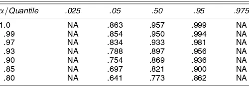
Table 1. The Panel Median-Unbiased Estimator: N=20, T+1=100, qit=ci+αqi, t−1+uit
nonmonotonic, near unity for very small values ofT. In a uni-variate context, Andrews (1993) reported that the .95 quantile function is hump-shaped in the vicinity of unity for small values ofTwhen a constant is not included in the regression. Phillips and Sul (2003) discussed this issue in a panel context. Their simulation evidence suggests that forN≥5 andT≥20, non-monotonicity of the median function is not an issue. In our subsequent empirical example, our dataset far exceeds these values ofN andT, and thus we will not have to worry about nonmonotonicity of the median function.
Our exactly median-unbiased estimators, as well as 90% and 95% CIs, are reported in Table 1. For comparison, Andrews’ (1993) exactly median-unbiased estimator forT+1=100 and
N=1 is given in Table 2.
Three interesting comparisons can be made between our panel median-unbiased estimator and Andrews’ univariate median-unbiased estimator. First, as in the univariate case, the panel estimates are downward-biased, with the bias more se-vere asα moves closer to unity. For example, whenα=.93, the panel estimator has a median bias of−.03, whereas when
α=.80, the median bias is−.004. Second, the median bias is not quite as severe in the panel DF regression as in the univari-ate DF regression. For example, whenα=.97, Andrews’ esti-mator has a median bias of−.037, whereas our panel estimator has a median bias of−.034. Third, the confidence intervals for our panel estimator are tighter than those for Andrews’ univari-ate estimator. These features accord with intuition. Correctly imposing the restriction thatαbe equal across equations is in-formation not available in a univariate context and should lead to an estimate closer to the true value. Similarly, when we esti-mate a system of equations and impose correct cross-equation restrictions, we achieve an increase in efficiency.
Turning now to approximately median-unbiased estimation of αin panel ADF regressions, we propose an ad hoc exten-sion of the univariate approximately median-unbiased estimator of Andrews and Chen (1994). Conditional onψ1i, ψ2i, . . . , ψkii
Table 2. The Andrews’ (1993) University Median-Unbiased Estimator: T+1=100, qt=c+αqt−1+ut
NOTE: Andrews (1993) reported only 90% confidence intervals. NA, not applicable.
Murray and Papell: Panels and Purchasing Power Parity 413
for i=1,2, . . . ,N, we calculate the approximately median-unbiased estimator ofαin the panel ADF regression,α1,AMU. Conditional onα1,AMU, we obtain new estimates of ψ1i, ψ2i,
. . . , ψkii that we use to calculate α2,AMU. αAMU is obtained when convergence occurs.
4. EMPIRICAL RESULTS
We now turn to the data. Our data consist of 20 quarterly U.S. dollar denominated real exchange rates for 1973:1–1998:2. These are the same data used by Murray and Papell (2002). The 20 countries are Australia, Austria, Belgium, Canada, Denmark, Finland, France, Germany, Greece, Ireland, Italy, Japan, The Netherlands, New Zealand, Norway, Portugal, Spain, Sweden, Switzerland, and the United Kingdom. We end the data in 1998:2, when the nominal exchange rates among the European countries became irrevocably fixed. Although there is a large literature on lag selection in univariate unit root tests, there is little guidance on how to choose the lag length in panel unit root regressions so that the resulting test has good size and power. We use the two most common methods of choosingk, the GS procedure of Hall (1994) and Ng and Perron (1995) and the MAIC of Ng and Perron (2001). We set the maximum lag at 12, the convention with quarterly data.
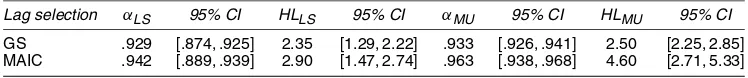
Our results are presented in Table 3. For the panel ADF re-gression with GS lag selection, the LS estimate ofαis .929, im-plying a half-life of 2.35 years. When the MAIC is used, we find a LS estimate of .942, corresponding to a half-life of 2.90 years. We have also supplemented these point estimates with paramet-ric bootstrap CIs. In the bootstrap, the covariance matrix of the errors is set to equal the covariance matrix of the LS residuals. The 95% bootstrap CI for the LS half-life is[1.29,2.22]years with GS lag selection and[1.47,2.74]years when the MAIC is used. Taken at face value, these CIs solve the PPP puzzle. The upper bounds are below the lower end of Rogoff’s consensus, and the lower bounds are consistent with half-lives implied by models with nominal rigidities. Notice, however, that the fail-ure of the bootstrap is so severe in this case that the 95% CIs lie entirely below the point estimates. This reflects the bias inher-ent in LS estimates ofαwhen the true value is close to unity. In addition, these bootstrap CIs have an additional layer of bias, because they reflect biased estimates based on a biased para-meterization (see Kilian 1998 for a discussion). These results suggest that the practice of bootstrapping LS half-life estimates in panel regressions with small samples should be avoided.
We now turn to correcting for median bias in panel ADF re-gressions. To allow for contemporaneous correlation, the co-variance matrix of the errors in our simulations is set equal to the covariance matrix of the LS residuals. Because our ADF re-gressions capture serial correlation, this framework allows for both serially and contemporaneously correlated errors. These results are also reported in Table 3. When GS lag selection
is used, we find an approximately median-unbiased estimate of α of .933, implying a half-life of 2.50 years. The 95% CI is [2.25,2.85] years. With MAIC lag selection, the approxi-mately median-unbiased estimate ofαis .963, implying a half-life of 4.60 years. The 95% CI in this case is[2.71,5.33]years. The differences between these CIs is, of course, due entirely to the chosen lag lengths. For this dataset, GS typically leads to a higher value ofkthan MAIC. Eight of the 20 exchange rates have values ofkin the range of 6–8. The lowest value ofk cho-sen by GS is 3. In contrast, the MAIC results in a much more parsimonious panel. Eleven of the 20 time series have k=0, and the largest value ofkchosen is 5. It is not surprising that the more parsimonious panel leads to a larger estimate of the half-life. Because there is no reason to prefer one of these CIs over the other, we consider the median of the two CIs, which is
[2.48,4.09]years. This interval is very close to Rogoff’s 3- to 5-year consensus. In particular, the lower bound is large enough to rule out economic models with nominal rigidities as can-didates for explaining the observed behavior of real exchange rates.
We again note that the estimated half-lives, and 95% CIs, are calculated directly fromαand are not based on an impulse re-sponse function. The reason for this is that ki andψij are not equal across countries in the panel. As such, there is no impulse response function for the entire panel. Calculating the half-life directly fromαis potentially problematic, because this as-sumes that shocks decay at a monotonic rate. For AR processes with k>1, shocks do not necessarily decay monotonically, so calculating half-lives based onα is potentially misleading. Nevertheless, previous research has demonstrated that for this dataset, there are only minor differences between calculating the half-life from ln(.5)/ln(α)and the impulse response func-tion. Murray and Papell (2002) reported univariate median-unbiased point estimates and CIs for half-lives based onαand the impulse response function for the dataset used here. The re-sults are strikingly similar. The point estimates for both meth-ods are very close, and the CIs are virtually identical. Therefore, we believe that computing the half-lives based on α for this dataset is not misleading.
To quantify the benefit of working in a panel context, we compare our results with their univariate counterparts. For the same dataset, Murray and Papell (2002) computed univariate half-lives using GS lag selection. When the half-life is com-puted directly from α, their median half-life CI is [.74,∞)
years. We have also redone Murray and Papell’s (2002) univari-ate approximunivari-ately median-unbiased estimunivari-ates (their table 8) us-ing the MAIC. We report these results in Table 4. The median 95% CI whenkis chosen by MAIC is [1.36,∞)years. Both of these CIs are so wide so as to be completely uninformative. The lower bounds of about 1 year are consistent with a rate of convergence to PPP that is predicted by models with nominal rigidities, and the upper bounds are consistent with the failure of PPP to hold in the very long run.
Table 3. Half-Lives in Panel Unit Root Regressions Quarterly Data: 1973:1–1998:2
Lag selection αLS 95% CI HLLS 95% CI αMU 95% CI HLMU 95% CI
GS .929 [.874, .925] 2.35 [1.29, 2.22] .933 [.926, .941] 2.50 [2.25, 2.85] MAIC .942 [.889, .939] 2.90 [1.47, 2.74] .963 [.938, .968] 4.60 [2.71, 5.33]
Table 4. Approximately Median-Unbiased Half-Lives in ADF Regressions. Quarterly Data: 1973:1–1998:2,
Why are our panel CIs so much tighter than their univariate counterparts? We can think of two potential explanations. First, panel tests have higher power than univariate tests because they exploit both cross-sectional and time series variability. Second, panel tests exploit the information contained in the contempo-raneous correlation of the real exchange rates. We investigate these explanations by conducting our panel median-unbiased simulations with contemporaneously uncorrelated errors. The median-unbiased half-life intervals with uncorrelated errors are
[2.66,8.58] years for GS and [3.60,10.74] years for MAIC. Although these CIs are narrower than their univariate coun-terparts reported in Table 4, they are wider than the CIs with contemporaneous correlation reported in Table 3. The gains in precision appear to come from both increasing power and al-lowing the errors to be contemporaneously correlated.
5. SUMMARY AND CONCLUDING REMARKS
By exploiting both cross-sectional and time series variabil-ity, panel methods offer the promise of sharpening the evidence of PPP over the post-Bretton Woods flexible exchange rate pe-riod. The purpose of this article is to evaluate the evidence that these methods help solve the “PPP puzzle” by shortening esti-mates of half-lives of PPP deviations.
The focus of this article is on the downward bias that LS methods impart to half-life estimates. We have extended the median-unbiased estimation methods of Andrews (1993) and Andrews and Chen (1994) to the panel context. We have shown that in general, panel methods are subject to the same bias problems as univariate methods and in particular, these bi-ases influence half-life estimates of PPP deviations. For panel ADF regressions that allow for serially and contemporaneously correlated errors, the bias in the LS estimates is so severe that the 95% bootstrap CIs for the half-life lie entirely below the point estimates.
Using approximately median-unbiased methods, the median 95% panel ADF CI for the half-life is[2.48,4.09]years, close to Rogoff’s 3- to 5-year consensus. It is worth remembering
that Rogoff’s survey consisted primarily of studies applying univariate methods to long-horizon data. Using panel methods and post-1973 data, we provide strong confirmation of his evi-dence of long half-lives of PPP deviations. However, panels do not help solve the PPP puzzle. Even the median lower bound of our 95% CIs (2.48 years) is, in Rogoff’s words, “seemingly far too long to be explained by nominal rigidities.”
ACKNOWLEGMENTS
The authors thank Lutz Kilian, Donggyu Sul, and two anony-mous referees for helpful comments and suggestions. Papell thanks the National Science Foundation for financial support.
[Received April 2003. Revised March 2005.]
REFERENCES
Abuaf, N., and Jorion, P. (1990), “Purchasing Power Parity in the Long Run,” Journal of Finance, 45, 157–174.
Andrews, D. W. K. (1993), “Exactly Median-Unbiased Estimation of First-Order Autoregressive/Unit Root Models,”Econometrica, 61, 139–165. Andrews, D. W. K., and Chen, H.-Y. (1994), “Approximately Median-Unbiased
Estimation of Autoregressive Models,”Journal of Business & Economic Sta-tistics, 12, 187–204.
Cheung, Y.-W., Chinn, M., and Fujii, E. (2001), “Market Structure and the Per-sistence of Sectoral Deviations From Purchasing Power Parity,”International Journal of Finance and Economics, 6, 95–114.
Choi, C.-Y., Mark, N. C., and Sul, D. (2004), “Unbiased Estimation of the Half-Life to PPP Convergence in Panel Data,”Journal of Money, Credit and Bank-ing, to appear.
Engel, C., and Morley, J. C. (2001), “The Adjustment of Prices and the Adjust-ment of the Exchange Rate,” working paper, University of Wisconsin. Fleissig, A. R., and Strauss, J. (2000), “Panel Unit Root Tests of Purchasing
Power Parity for Price Indices,”Journal of International Money and Finance, 19, 489–506.
Hall, A. (1994), “Testing for a Unit Root in Time Series With Pretest Data-Based Model Selection,”Journal of Business & Economic Statistics, 12, 461–470.
Im, K. S., Pesaran, M. H., and Shin, Y. (2003), “Testing for Unit Roots in Het-erogeneous Panels,”Journal of Econometrics, 115, 53–74.
Imbs, J., Mumtaz, H., Ravn, M., and Rey, H. (2005), “PPP Strikes Back: Aggre-gation and the Real Exchange Rate,”Quarterly Journal of Economics, 120, 1–43.
Murray and Papell: Panels and Purchasing Power Parity 415
Kilian, L. (1998), “Small-Sample Confidence Intervals for Impulse Response Functions,”Review of Economics and Statistics, 80, 218–230.
Levin, A., Lin, C. F., and Chu, J. (2002), “Unit Root Tests in Panel Data: Asymptotic and Finite-Sample Properties,”Journal of Econometrics, 108, 1–24.
Lothian, J., and Taylor, M. (1996), “Real Exchange Rate Behavior: The Recent Float From the Perspective of the Past Two Centuries,”Journal of Political Economy, 104, 488–509.
Murray, C. J., and Papell, D. H. (2002), “The Purchasing Power Parity Persis-tence Paradigm,”Journal of International Economics, 56, 1–19.
(2005), “The Purchasing Power Parity Puzzle Is Worse Than You Think,”Empirical Economics, to appear.
Ng, S., and Perron, P. (1995), “Unit Root Tests in ARMA Models With Data-Dependent Methods for the Selection of the Truncation Lag,”Journal of the American Statistical Association, 90, 268–281.
(2001), “Lag Length Selection and the Construction of Unit Root Tests With Good Size and Power,”Econometrica, 69, 1519–1554.
Obstfeld, M. (2001), “International Macroeconomics: Beyond the Mundell– Flemming Model,”International Monetary Fund Staff Papers, 47, 1–39.
Papell, D. H. (1997), “Searching for Stationarity: Purchasing Power Parity Un-der the Current Float,”Journal of International Economics, 43, 313–332.
(2002), “The Great Appreciation, the Great Depreciation, and the Pur-chasing Power Parity Hypothesis,”Journal of International Economics, 57, 51–82.
Papell, D. H., and Theodoridis, H. (2001), “The Choice of Numeraire Currency in Panel Tests of Purchasing Power Parity,”Journal of Money, Credit and Banking, 33, 790–803.
Phillips, P. C. B., and Sul, D. (2003), “Dynamic Panel Estimation and Homo-geneity Testing Under Cross-Section Dependence,”The Econometrics Jour-nal, 6, 217–260.
Rogoff, K. (1996), “The Purchasing Power Parity Puzzle,”Journal of Economic Literature, 34, 647–668.
Taylor, A. M. (2001), “Potential Pitfalls for the Purchasing-Power-Parity-Puzzle? Sampling and Specification Biases in Mean-Reversion Tests of the Law of One Price,”Econometrica, 69, 473–498.
Wu, Y. (1996), “Are Real Exchange Rates Nonstationary? Evidence From a Panel-Data Test,”Journal of Money, Credit and Banking, 28, 54–63.