Full Terms & Conditions of access and use can be found at
http://www.tandfonline.com/action/journalInformation?journalCode=ubes20
Download by: [Universitas Maritim Raja Ali Haji] Date: 12 January 2016, At: 00:14
Journal of Business & Economic Statistics
ISSN: 0735-0015 (Print) 1537-2707 (Online) Journal homepage: http://www.tandfonline.com/loi/ubes20
Model-Based Clustering of Non-Gaussian Panel
Data Based on Skew-t Distributions
Miguel A. Juárez & Mark F. J. Steel
To cite this article: Miguel A. Juárez & Mark F. J. Steel (2010) Model-Based Clustering of Non-Gaussian Panel Data Based on Skew-t Distributions, Journal of Business & Economic Statistics, 28:1, 52-66, DOI: 10.1198/jbes.2009.07145
To link to this article: http://dx.doi.org/10.1198/jbes.2009.07145
Published online: 01 Jan 2012.
Submit your article to this journal
Article views: 192
View related articles
Model-Based Clustering of Non-Gaussian Panel
Data Based on Skew-
t
Distributions
Miguel A. JUÁREZ
and Mark F. J. STEEL
Department of Statistics, University of Warwick, CV4 7AL Coventry, U.K.
(M.A.Juarez@warwick.ac.uk;M.F.Steel@stats.warwick.ac.uk)
We propose a model-based method to cluster units within a panel. The underlying model is autoregressive and non-Gaussian, allowing for both skewness and fat tails, and the units are clustered according to their dynamic behavior, equilibrium level, and the effect of covariates. Inference is addressed from a Bayesian perspective, and model comparison is conducted using Bayes factors. Particular attention is paid to prior elicitation and posterior propriety. We suggest priors that require little subjective input and have hierarchi-cal structures that enhance inference robustness. We apply our methodology to GDP growth of European regions and to employment growth of Spanish firms.
KEY WORDS: Autoregressive modeling; Employment growth; GDP growth convergence; Hierarchical prior; Model comparison; Posterior propriety; Skewness.
1. INTRODUCTION
Models for panel or longitudinal data are used extensively in economics and related disciplines (Baltagi2001; Hsiao2003), as well as in health and biological sciences (Diggle et al.2002; Weiss 2005). Typically, panels are formed according to some criteria (e.g., geographical, economical, demographical), with the intention of gaining strength when estimating quantities common to all individual units in the panel. But this group-ing may strongly affect inference if presumed common char-acteristics of the units are actually quite different. In these cases, clustering units within the panel may prove useful. This will allow the units to share some common parameters, thus borrowing strength in their estimation, but to also have some cluster-specific parameters. In particular, we consider model-based clustering, which is model-based on a formal statistical frame-work (Banfield and Raftery1993; Fraley and Raftery2002). In an economic context, Bauwens and Rombouts (2007) proposed a method for clustering many generalized autoregressive condi-tional heteroscedasticity models, whereas Frühwirth-Schnatter and Kaufmann (2008) discussed a Bayesian clustering method for multiple time series data. From a frequentist perspective, Lin and Ng (2007) proposed nonparametric model-based clus-tering methods for panel data with fixed effects.
Even though the majority of the literature uses Gaussian models, it is often the case that data contain outliers, which can be dealt with by allowing for heavier-than-normal tail behavior, as well as asymmetries, which require the underlying distribu-tion to allow a certain amount of skewness. The former issue is frequently addressed by assuming a Student distribution withν degrees of freedom (denoted here bytν), usually withν fixed
at a small value. In comparison, there has been much less de-velopment in dealing with asymmetry. Hirano (2002) proposed a semiparametric framework, with a nonparametric distribution on the error term, using a Dirichlet prior. In this article we use fully parametric yet flexible models, based partly on the models of Juárez and Steel (2009), that allow for clustering and addi-tional covariates, and conduct inference from a Bayesian view-point.
Because the aims of this article are rather similar to those of Frühwirth-Schnatter and Kaufmann (2008), we briefly
high-light the differences with the approach that those authors used. First, our modeling allows for skewness and imposes station-arity In addition, we use shrinkage within the clusters only for the equilibrium levels, whereas we pool for the autoregressive coefficients. Frühwirth-Schnatter and Kaufmann (2008) either shrank or pooled both (although Frühwirth-Schnatter and Kauf-mann2006pooled only part of the parameters in a somewhat related model). The prior that we used in this work is carefully elicited and is improper, unlike the conditionally natural conju-gate prior used by Frühwirth-Schnatter and Kaufmann (2008). This implies that we need to make sure that the posterior exists (we derive a simple and easily verifiable condition for propri-ety), but we need to elicit fewer hyperparameters, and, more importantly, our prior enjoys a natural invariance (for the para-meter on which we are improper) with respect to affine transfor-mations of the data, which leads to desirable robustness proper-ties. In addition, we reduce the dependence of the Bayes factors on prior assumptions by using hierarchical prior structures. Fi-nally, we allow for the data to inform us on the tails of the error distribution, because we keepνa free parameter.
An important contribution of this article is the introduction of a flexible model that can be applied in a wide variety of eco-nomic contexts with a “benchmark” prior that will be a reason-able reflection of prior ideas in many applied situations. Thus our aim is to provide a more or less “automatic” Bayesian pro-cedure that can be used by applied researchers without sub-stantial requirements for prior elicitation. The prior structure asks the user for a mean and a variance of the parameters de-scribing long-run equilibrium levels and allows for compari-son (or averaging) of models with different numbers of clusters through Bayes factors. Priors on the model-specific parameters are given a hierarchical structure. This leads to greater flexi-bility and, more importantly, reduces the dependence of pos-terior inference and especially Bayes factors on prior assump-tions, thus inducing a larger degree of robustness. Matlab code that implements the methodology described in this article is
© 2010American Statistical Association Journal of Business & Economic Statistics
January 2010, Vol. 28, No. 1 DOI:10.1198/jbes.2009.07145
52
freely available athttp:// www.warwick.ac.uk/ go/ msteel/ steel_ homepage/ software/, along with the data sets used in the appli-cations.
The rest of the article is organized as follows. Section2 de-scribes the model and discusses the prior specification and pos-terior propriety. Section3briefly discusses numerical methods for conducting inference with this model. Section4 discusses the analysis of simulated data, which are used to assess the model performance in terms of clustering. Section5 analyzes two real data sets to illustrate implementation of the model: one comprising per capita GDP growth data for European regions and the other describing employment growth in Spanish manu-facturing firms. Section6presents some concluding remarks.
2. THE MODEL
Assume that the available data,y= {yit}, form a (possibly un-balanced) panel ofi=1, . . . ,mindividuals, for each of which we haveTiconsecutive observations. In addition, we observe a vector,xit=(x1it, . . . ,x
p
it)′, of covariates. We focus on the first-order autoregressive model
yit=βi(1−α)+αyit−1+(1−α)µxit+λ−1/2εit, (1) where the errors{εit}are independent and identically distrib-uted random quantities with mode at zero and unit precision, αis the parameter governing the dynamic behavior of the panel, andµ=(μ1, . . . , μp)is a vector of coefficients related top ex-planatory variables inxit. We assume that the process is sta-tionary, i.e.,|α|<1. The parametersβi are individual effects. Because the error distribution has zero mode, these individual effects can be interpreted as reflecting differences in the long-run modal tendencies for the corresponding individuals. In ad-dition, the individual effects are assumed to be related accord-ing to βi∼N(βi|β, τ−1), which is a commonly used normal random-effects specification (found in, e.g., Liu and Tiao1980; Nandram and Petruccelli1997; Gelman 2006), where β is a common mean andτ is the precision. Within a Bayesian frame-work, this is merely a hierarchical specification of the prior on theβi’s, which puts a bit more structure on the problem and al-lows us to parameterize the model in terms ofβ andτ, rather than allmindividual effects. Finally, we condition throughout on the initial observed values,yi0, and assume that the process
started a long time ago.
To accommodate skewness while retaining a unique mode at zero, we assume that the error term follows a skew distribution as in Fernández and Steel (1998). Thus, given a unimodal prob-ability density functionf that has support on the real line and is symmetric around zero, we consider
is the skewness parameter. Clearly, forγ=1, the density sim-plifies tof, and forγ =1, we have skewness, characterized by P(x>0|γ )=γ2/(1+γ2). Positive skewness corresponds to γ >1, whereas negative skewness is generated byγ ∈(0,1). Fernández and Steel (1998) derived an explicit expression for the moments in terms of the moments off. Of course, we could introduce skewness in other ways, such as done by Jones and Faddy (2003) and Azzalini and Capitanio (2003), but we pre-fer the approach adopted here because it retains a zero mode
and because of its inferential simplicity and the clear interpre-tation of the extra parameterγ. The latter also facilitates prior elicitation.
To also allow for fat tails, we focus on skew versions of the Student-tν distribution, leading to
where the degrees of freedomνis treated as a free parameter. The basic model then consists of (1) withεitdistributed ac-cording to (3). In this model, we can clearly interpretαas the parameter governing the dynamics of the panel,λas the obser-vational precision,βias the individual long-run level, andµas a measure of the long-run modal effect of the covariates on the observable. In addition,γ controls the skewness, andν deter-mines the tail behavior.
As discussed earlier, pooling similar time series can be ben-eficial when estimating a model, but when the behavior is not sufficiently homogeneous, the resulting pooled estimates may be misleading, as we will illustrate in the applications in the se-quel. Clustering is one way to maintain the advantages of pool-ing while also allowpool-ing for heterogeneity within the panel (see, e.g., Canova2004; Frühwirth-Schnatter and Kaufmann 2008; Hoogstrate, Palm, and Pfann 2000). To allow for clustering within the panel, we assume that all units share a common pa-rameter vector, say,θC, and that each has a cluster-specific set of parameters inθj, forj=1, . . . ,K, whereKis the number of clusters in the panel.
Specifically, we assume that the different behavior may arise either from the dynamics, the coefficients of the covariates, or from the equilibrium level of the series. So extending (1) to allow for different dynamics, covariate effects, and levels for each cluster yields
yit=βi(1−αj)+αjyit−1+(1−αj)µjxit+λ−1/2εit, (4) with|αj|<1 and
βi∼N(βi|βj, τ−1); j=1, . . . ,K. (5) ThusθC= {γ , ν, λ, τ}andθj= {αj, βj,µj}. The interpretation of the cluster-specific parameters is as follows. αj character-izes the autoregressive dynamics, whereas the long-run average equilibrium level is given byβj, provided that we standardize xitto have mean 0 for each unit. Finally, the equilibrium level at each time point also will depend onxitthrough the coefficients inµj.
Note that we have specified common values for the preci-sions in (4) and (5), as well as the nonnormality parameters of the error distribution in (3). This reflects both our judgment that these are unlikely to be parameters of interest and that learning about the nonnormality parameters, especiallyν, from the data is relatively difficult. Making more parameters cluster-specific is perfectly feasible, but we feel the current specification is a good way to focus attention on differences between the clus-ters that we can easily interpret. Finally, we also can consider alternative partitions of the parameters, where, for example, only the dynamics are cluster-specific, that is, the model with βj=β,µj=µ,j=1, . . . ,K, leading toθC= {β,µ, γ , ν, λ, τ}, andθj=αj.
2.1 Prior Specification of which we discuss in the next section.
We adopt a standard diffuse (improper) prior for λ, which is invariant with respect to affine transformations. Theorem1
provides a simple condition for posterior existence under this improper prior. For τ, however, we need a proper prior, and we adopt a gamma distribution with shape parameter 2 and a scale consistent with the observed between-group variance of the group (i.e. individual) means,s2β, by making the prior mode equal to 2/s2β; this distribution is denoted by Ga(2,s2β/2). The prior onγ is induced by a uniform prior on the skewness mea-sure defined as 1 minus twice the mass to the left of the mode. Full details and further motivation for these choices were pro-vided by Juárez and Steel (2009). Thus we adopt
π(λ)∝λ−1, (7)
τ ∼Ga(2,s2β/2), (8) π(γ )=2γ (1+γ2)−2. (9) Because the degrees of freedom parameterνoften is not clearly determined by the data, we consider three different priors. First, we take a Ga(2,1/10)prior forν with mass covering a large range of relevant values (prior mean 20 and variance 200). This prior leads to the probability density function (pdf)
π1(ν)= ν
100exp[−ν/10], (10) which has a mode at 10 and allows for all prior moments to exist. We also consider a hierarchical prior by taking an expo-nential prior on the scale parameter of a gamma distribution with shape parameter 2, which leads to the pdf
π2(ν)=2d ν
(ν+d)3. (11)
This introduces a parameter d>0, which controls the mode (d/2) and the median ((1+√2)d). The tail is now too heavy to allow for a mean. Finally, in the context of Studenttregression models, Fonseca, Ferreira, and Migon (2008) derived a Jeffreys prior forν that has an “objective” flavor and performs well in terms of frequentist coverage. This prior is proper with pdf
π3(ν)∝
whereψ′(·)is the trigamma function. This prior has the same right-tail behavior asπ2, not allowing for a mean, but has quite
different behavior close to zero, because it is unbounded asν tends to zero. The median is always equal to 0.55; thus the prior onνis given by one of (10), (11), or (12).
We also need to specify a prior on the assignment of units to clusters. A common approach is to augment the data with the
indicator variableSi∈ {1, . . . ,K}, whereSi=jmeans that uniti belongs to clusterj. Thus we can write
f(yi|Si,θ)=f(yi|θj,θC) forSi=j,j=1, . . . ,K, whereθ=(θC,θ1, . . . ,θK).
A priori, we assume that, independently,
P[Si=j|η] =ηj,
where ηj is the relative size of cluster j = 1, . . . ,K and
η=(η1, . . . , ηK)′. Obviously, η′ι=1 (where ι denotes a K-dimensional vector of 1’s), and thus it is natural to specify the Dirichlet priorπ(η)=Di(η|e), where we use a “Jeffrey’s type” prior withe=(1/2)×ι (see Berger and Bernardo 1992). In addition, we exclude from the sampler cluster assignments that do not lead to a proper posterior (as we explain in Sec.2.3). Therefore, the joint prior forS= {S1, . . . ,Sm}andηis
whereI(S)is 1 if the assignment gives rise to a proper posterior and 0 otherwise.
2.2 The Prior on the Cluster-Specific Parameters
An important reason for wanting to put a carefully elicited proper prior on cluster-specific parameters is that we typically want to compute Bayes factors between models with different numbers of components. If the components have, say, a com-monβandµ, then this will be perfectly feasible with a flat im-proper prior on(β,µ), but in the general case whereβj’s and/or
µj’s are cluster-specific, such Bayes factors will no longer be defined. Of course, any proper prior on the cluster-specific pa-rameters inθjwill give us Bayes factors, but we need to be very careful that the prior onα,β, andM truly reflects reasonable prior assumptions, because the Bayes factors will depend cru-cially on the particular prior used.
Within each cluster, the dynamics parameterαgets a rescaled Beta prior [on(−1,1)], and we make the hyperparameters of this Beta distribution random, with equal gamma priors. This hierarchical structure of the prior onαleads to more flexibility. In particular, we adopt
The implied marginal prior onα is roughly bell-shaped with P(|α| <0.5)=0.65 and P(|α| >0.9)=0.03, in line with reasonable prior beliefs for our (and most) applications. In the context of our clustering model, we use independent and identical priors for the dynamics parameters. Thus, defining aα= (aα1, . . . ,aαK)′andbα= (bα1, . . . ,bαK)′, we have
where each component prior is specified as before. Note that this hierarchical prior structure onαwill make the Bayes fac-tors between models with different K less dependent on the prior assumptions.
The long-run equilibrium levels associated with each cluster often are quantities about which we have some prior informa-tion. Within the product form of (6), we propose the following multivariate normal prior forβ:
β∼NKβ|mι,c2[(1−a)I+aιι′], (18) wherec>0 and−1/(K−1) <a<1. The prior in (18) gen-erates an equicorrelated prior structure for β with prior cor-relationa throughout. Thus if a=0, then we have indepen-dent normally distributedβj’s, but ifa→1, then they tend to perfect positive correlation. The main reason for allowing for nonzeroa becomes clear when we consider that (18) implies that βj ∼N(m,c2),j=1, . . . ,K and βi−βj∼N(0,2c2(1−
a)),i=j,i,j=1, . . . ,K. Thus fora=0, the prior variance of the difference between the equilibrium levels of two clusters would be twice the prior variance of the level of any cluster. This would seem to be counterintuitive, and positive values of awould be closer to most prior beliefs. In fact,a=3/4, leading to var(βi−βj)=(1/2)×var(βj), might be more reasonable.
Because we typically will have a fair amount of sample infor-mation onβj, we can go one step further and, rather than fixing aat, say, a reasonable positive value, we can keeparandom and put a prior on it. This implies an additional level in the prior hi-erarchy and would allow us to learn aboutafrom the data. We put a beta prior ona, rescaled to the interval(−1/(K−1),1), and posterior inference onathen provides valuable information regarding the assumption that allβj’s are equal. In particular, if we find a significant amount posterior mass close to 1 fora, this would imply that a model withβj=β,j=1, . . . ,K(where only theαj’s andμj’s differ across clusters) might be preferable to the model with cluster-specificβj’s.
We specify a similar prior structure on the coefficientsM. So that we can interpret these coefficients, we standardize each of thepcovariates to have mean 0 and variance 1 for each individ-ual unit. Then we set the mean of the prior at0and use a similar covariance structure for theKcluster-specific coefficients of re-gressorl, grouped inµl=(μ1l, . . . , μKl )′, leading to
µl∼NKµl|0,c2l[(1−al)I+alιι′], l=1, . . . ,p, (19) where we choosecl>0 and specify a rescaled beta prior for eachal∈(−1/(K−1),1).
As an important bonus of such a hierarchical prior structure, the sensitivity of the Bayes factors to the prior assumptions will be greatly reduced. For example, in the model with cluster-specificβj’s, Bayes factors between models with different K depend on the prior onβ mostly through the implied prior on the contrastsβi−βj. If the priorπ(βi−βj)is unreasonably vague (corresponding toa very far from 1), then we will tend to favor smaller values ofK, whereas for excessively precise π(βi−βj)(i.e.avery close to 1), Bayes factors will point to models with more components. Thus, by changinga, we can af-fect model choice, and makingalargely determined by the data reduces the dependence of Bayes factors on prior assumptions. The prior in this section is similar to that specified by De-schamps (2006) for the regression coefficients in a Markov switching model, although there the same prior also was used for the dynamics parameters (thus precluding stationarity).
2.3 Propriety of the Posterior
Note that because (7) yields an improper joint prior, we need to verify the existence of the posterior.
Theorem 1. Consider the model defined by (4) and (5), with the error term distributed according to (3) and the prior spec-ification as described in Sections2.1and2.2. The posterior is proper if and only if Tj>mj+p+1 holds for at least one j=1, . . . ,K.
The condition of Theorem1is so weak that any sample with at least one unit with more thanp+2 observations will always lead to a proper posterior. Because the prior is improper only on the precisionλ, the existence of the posterior can be destroyed only by having so few observations that we can find a perfect fit in all clusters. As long as we have one cluster in which we can-not fit the data perfectly, we have a valid Bayesian analysis. Be-cause there are no cluster-specific parameters with an improper prior, empty clusters will not preclude Bayesian inference. We impose the condition in Theorem1in the sampler by truncating the prior in (13) throughI(S).
If we assume a common levelβj=βand/or a commonµj= µ, then the existence condition of Theorem1will continue to hold, because it is a necessary condition for integrating out the precisionλ.
In fact, we also can prove existence under improper flat pri-ors onβ andM under a slightly stronger condition. More de-tails and proofs of these results are provided in an earlier ver-sion of this article available at http:// www.warwick.ac.uk/ go/ msteel/ steel_homepage/ techrep/ clustnew.pdf.
3. MODEL ESTIMATION
There is a large literature on mixture models (see, e.g., Titter-ington, Smith, and Makov1985and McLachlan and Peel2000). Diebolt and Robert (1994), Marin, Mengersen, and Robert (2005), and, in particular, Frühwirth-Schnatter (2006) have pro-vide exhaustive discussions from the Bayesian perspective.
3.1 Likelihood
Augmenting the data with cluster indicatorsSias described earlier, we can write the likelihood as
L(θ,S)=
and wherefN(x|μ, ζ−1)is the pdf of a normal distribution onx with meanμand precisionζ.
In the foregoing sampling density, we use the representation of the Student distribution as a gamma-scale mixture of nor-mals (see Geweke 1993), which facilitates the computations. We will augment this with the mixing variablesωit in the sam-pler. We also have integrated the sampling density in (4) with the random-effects distribution in (5). Again, we will include the individual effectsβiin the sampler, which is computation-ally convenient and also allows for inference on each unit’s in-dividual effect.
Because analytic solutions for this mixture model are not available, we resort to Monte Carlo techniques, described briefly in the next section. When dealing with an unknown number of clusters, one of two alternative approaches may be followed: direct estimation in the sampler or model compari-son. The first of these, which involves a Markov chain mov-ing in spaces of different dimensions, was implemented by, for example, Green (1995) and Richardson and Green (1997) through reversible-jump Markov chain Monte Carlo, whereas Stephens (2000a) and Phillips and Smith (1996) proposed al-ternative samplers that move between models. We adopt the second approach; fitting the model for different values ofKand then computing Bayes factors to determine which number of clusters performs best, as was done by Bensmail et al. (1997), Frühwirth-Schnatter and Kaufmann (2008), and Raftery (1996). This approach is particularly useful in cases where the clusters have a specific interpretation, because inference given a chosen number of components is immediately available.
3.2 Computational Implementation
To conduct inference, we use Markov chain Monte Carlo (MCMC) methods, as is now common in the Bayesian litera-ture on finite mixlitera-ture models. Because most of the ideas can be found in the literature (see, e.g., Bensmail et al.1997; Marin, Mengersen, and Robert2005, and Frühwirth-Schnatter2006), we do not provide much detail here. We block the sampler into separate steps for each of the (vector) parameters and use Gibbs steps for the precisionsλandτ, the membership prob-abilities and indicatorsηandS, and the auxiliary mixing vari-ables{ωit}. The long-run equilibrium parametersβ andMare drawn with random-walk Metropolis steps with independentt3
proposals, with the scale chosen so as to obtain an appropriate acceptance rate. For all other parameters, we use Metropolis– Hastings steps from proposals with the mode equal to the pre-vious draw, tuning the free parameter to achieve the desired acceptance rates. We adopt independent rescaled Beta propos-als for the components of the dynamics parameterα and the correlationsa and{al}. We use independent gamma proposal distributions for the dynamics hyperparametersaα andbα, the
skewness parameterγ, and the degrees of freedomν.
As pointed out by Celeux, Hurn, and Robert (2000), Stephens (2000b), and Casella, Robert, and Wells (2004), a number of difficulties may arise when constructing a sampler for a mix-ture model. In particular, we need to take into account the multimodality of the posterior distribution caused by the in-variance under permutation of the cluster labels. To overcome this problem, Diebolt and Robert (1994) proposed imposing identifiability constraints, whereas Celeux, Hurn, and Robert
(2000) and Stephens (2000b) used decision-theoretical criteria. Casella, Robert, and Wells (2004) suggested a method based on an appropriate partition of the space of augmented variables. Casella et al. (2002) introduced a perfect sampling scheme, which is not easily extended to nonexponential families. Using the analytical structure of the posterior distribution, Frühwirth-Schnatter (2001) proposed a random permutation scheme, whereas Geweke (2007) introduced the permutation-augmented simulator, a deterministic modification of the usual MCMC sampler. Comprehensive discussions have been given by Jasra, Holmes, and Stephens (2005) and Frühwirth-Schnatter (2006).
In our setting, we are interested in differentiating between the components in terms of dynamics, long-run behavior, or co-variate effects. It would not be meaningful to distinguish be-tween the clusters in terms of the weightsηj. Thus we propose considering scatterplots of all of the draws on(α,β,M)before deciding on the labels. This will suggest which of the sets of parameters (α,β, or M) are best separated between the clus-ters, and we use the one that provides the clearest separation to identify the labels through an order constraint. This can then be done by simply postprocessing the MCMC output. In both of the real-data examples in this article, this indicates that impos-ing an identifiability constraint through the dynamics parame-ter,α, is a natural way to identify the labels.
To perform model comparison, we use the formal tool of Bayes factors. Posterior odds between any two models are then obtained immediately by multiplying the prior odds with the appropriate Bayes factor. These then can be used for either model comparison or Bayesian model averaging (for inference on quantities that are not model-specific, such as predictive in-ference). The Bayes factor between any two models is defined simply as the ratio of the marginal likelihoods. The marginal likelihood is the sampling density integrated out with the prior and is not immediately obtained from MCMC output. Several ways of approximating the marginal likelihood are available in the literature (see, e.g., Chib1995; DiCiccio et al.1997; New-ton and Raftery1994; and references therein). But in our case, these methods may yield poor results, due to the potential mul-timodality of the posterior. Steele, Raftery, and Emond (2006) and Ishwaran, James, and Sun (2001) have provided alterna-tive methods specifically designed for mixture models. Here we compute the marginal likelihood based on a particular permu-tation of the cluster labels, obtained from postprocessing the output as explained earlier. This implies that we need to correct the marginal likelihood by a factorK!(the number of possible permutations), because we have effectively underestimated the prior density by the same factor. As explained by Frühwirth-Schnatter (2004), this leads to a very precise estimate for well-separated clusters. In the case where the clusters are less well separated, the appropriate correction factor will be in(1,K!), and this procedure will give us an upper bound to the actual marginal likelihood. More precise estimation for such cases can be based on the method proposed by Frühwirth-Schnatter (2004), but this would not change any conclusions in the appli-cations studied here.
In the sequel, we will compute the marginal likelihood using the bridge sampler of Meng and Wong (1996). This method was used and extensively discussed by Frühwirth-Schnatter (2004) in a related context. DiCiccio et al. (1997) and Frühwirth-Schnatter (2006) have provided comprehensive discussions.
Bridge sampling generalizes importance sampling and com-bines sampling from the posterior distribution with that from an importance function. The marginal likelihood can be approxi-mated by a ratio of sample averages; one from the importance function and another from the posterior. These sample aver-ages both involve a so-called bridge function, which needs to be chosen subject to an integrability constraint. An important advantage of bridge sampling is its robustness with respect to the relative tail behaviour of the importance function. Given the complexity of the target distribution, which will potentially have heavy tails and be skewed, we construct the importance function using Studentt3 distributions, centered at the modal
MCMC values, for parameters with support onℜ; gamma den-sities with parameters matching the first two moments of the MCMC output, for positive parameters; and rescaled Beta dis-tributions, with parameters matching the first two moments of the chain, for the dynamics parameter, as well as the correla-tionsaof (18) andalof (19). The variance of these distributions is then doubled to facilitate sampling from the entire posterior support. This choice is intended to closely mimic the poste-rior, while still allowing for easy sampling from the importance density.
In the particular case where one model is a simple paramet-ric restparamet-riction of another model, we often can compute Bayes factors through the Savage–Dickey density ratio, which is the ratio of the posterior and the prior density values at the restric-tion (see Verdinelli and Wasserman 1995). For example, the Bayes factor in favor of a symmetric model over its skewed counterpart will bep(γ =1|data)/p(γ =1). This way of com-puting Bayes factors is typically easier and can be more pre-cise than using the methods estimating the marginal likelihoods mentioned earlier, but it is not always applicable, for example, when the restriction corresponds to a boundary or limit of the parameter space.
4. SIMULATED DATA AND CLUSTERING PERFORMANCE
On the basis of various simulated data sets, we conclude that the numerical methods work well and that the prior described in Sections2.1and2.2is reasonable and not overly informative. Inference based on both simulated and real data demonstrates very little difference among the three different priors forν. In particular, none of the results reported here was noticeably af-fected by this prior choice. The only difference that we iden-tified was for situations where the data are close to normality, due to the variations in right tail behavior. In particular, the sam-pler then mixes less well with the fatter-tailed priorsπ2(ν)and π3(ν), due to the combination of a relatively flat likelihood and
a very fat prior tail. Because any value ofνabove 50 or so is practically indistinguishable from normality, we are not too in-terested in minor differences in the far right tail, and thus we report only results with the priorπ1(ν)in the sequel.
We now use simulated data to highlight the model’s ability to correctly identify the clusters. This will enhance our under-standing of the model’s properties and limitations.
Data were generated from the following baseline model. We takeK=2, m=80,T =10, andyi0=0 for alli=1, . . . ,m.
Note that we do not start from “equilibrium” conditions, mak-ing it more challengmak-ing for the model to adequately cluster in terms ofβ. A total ofp=3 covariates were generated from a
uniform distribution and then standardized. We use the parame-ter values
which means the clusters are always distinguished by a very small difference in M. Throughout, membership probabilities are{0.3,0.7}.
The prior that we used is as described in Sections2.1and2.2, withm=0 andc=0.3 in (18),cl=1 in (19), and a uniform prior on correlationsaandal.
With these simulated data, we ran MCMC chains of 50,000, discarding the first 10,000 and recording every 10th draw. The computational cost for each chain was about 1.4 hours of CPU time using our Matlab code on a single-core Xeon processor with a clock speed of 3 GHz. (We could run up to four runs in parallel using a workstation with two processors.) Running considerably longer chains led to virtually identical results.
4.1 Effect of the Error Distribution
An interesting question is whether the non-Gaussian error distribution has a large effect on our estimates. We generate data from the skew-tmodel described earlier. To further distin-guish between the clusters, we takeα=(0.1,0.3)′, whereas we use identical long-run levelsβ=(0.02,0.02)′. Posterior infer-ence on the parameters using the correct skew-tmodel is well concentrated around the values used to generate the data with a relatively small spread. Neglecting fat tails mostly affects the inference on the observational precision,λ, as can be expected. Neglecting skewness by estimating the usual Gaussian model has an additional large effect on the equilibrium levels, which are shifted downward by>60% of the length of the 95% credi-ble intervals (CIs). (Throughout, CIs are taken from the 2.5th to the 97.5th percentiles.) Again, this is as expected, because we attempt to capture a negatively skewed distribution (γ <1) by a symmetric one, which will underestimate the mode.
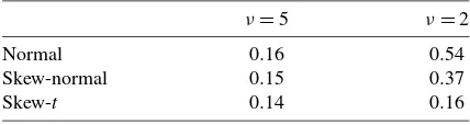
To assess the classification performance, we consider the av-erage probability of misclassification, defined as P(Si=j|yi is generated by clusterj)averaged over allmunits. Table1 sum-marizes our findings for these data, as well as another data set generated as before but with ν=2 (which is not an unusual value in light of our real data applications later). Clearly, not accounting for either of the non-Gaussian aspects of the error distribution worsens the clustering performance, especially for ν=2.
Table 1. Synthetic skewed and fat-tailed data: Average misclassification probabilities for each model using two different data sets (generated with different tail behaviors)
ν=5 ν=2
Normal 0.16 0.54
Skew-normal 0.15 0.37
Skew-t 0.14 0.16
4.2 Effect of the Distance Between Clusters
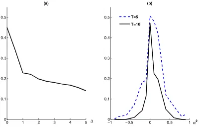
We examine two ways in which the clusters differ. First, we fix the dynamics parameters at 0.1 and vary the equilibrium lo-cations by takingβ1=0 and varyingβ2. We express the nor-malised difference as=τ1/2(β2−β1). Figure1(a) shows the average probability of misclassification, as defined earlier. We see that the ability to correctly classify the data improves with increasing distance between the clusters, as expected. Despite the fact that the data for both clusters have the same starting value, we already have a significant improvement in the clus-tering ability when the long-run levels are one (random effect) standard deviation apart.
We then fix β1=β2=0.02 and α1=0 and let α2 vary. Figure 1(b) shows that we can distinguish the clusters for α2<−0.2 or α2>0.4 quite accurately. In this case we also repeat the experiment with a smaller time dimension,T=5. Of course, this diminishes the model’s performance somewhat, but we still have quite good clustering properties for values ofα2 far away from the extremes. In both samples, it appears to be easier to identify the clusters for a given|α2|ifα2<0, because the implied alternating behavior is quite noticeable.
5. APPLICATIONS
In this section we report an analysis of two real data sets. The first data set comprises the per capita GDP of European regions, similar to that used by Canova (2004) and Frühwirth-Schnatter and Kaufmann (2008). Here we focused on annual GDP growth. The second data set is a panel of 738 Spanish manufacturing firms, taken from Arellano (2003, sec. 6.7), for which we modeled growth of employment.
We used the prior discussed in Sections 2.1 and 2.2. The induced prior on each long-run growth level βj was N(0.05, 0.052)for the GDP data and N(0,0.052)for the firms example.
For the GDP growth data, we used a covariate, the (standard-ized) level of GDP in the previous period, for which the prior ofμjwas N(0,1). For the correlation parametersaof (18) and alof (19), we used a uniform prior over(−1/(K−1),1)in both applications.
We ran MCMC samplers for 170,000 iterations, discarding the first 20,000 and then taking every 10th draw, ending up with an effective size of 15,000. This required roughly 13 hours and 19.5 hours on a single-core 3-GHz Xeon processor for the two applications.
5.1 Per capita Income of European Regions
There is a vast literature concerned with economic growth and convergence. Although there apparently is no empirical evidence of overall growth convergence (Durlauf and Johnson
1995; Durlauf and Quah1999; Temple1999), some clusters of homogeneous growing countries/regions or convergence clubs have been found (see, e.g., Canova2004; Quah1997). Pesaran (2007), using data from the Penn World Tables, found evidence against convergence in levels but in favor of convergence in growth rates.
Here we concentrated on annual per capita GDP growth rates from 258 NUTS2 European regions for the period 1995–2004. The NUTS Classification (Nomenclature des Unités Territori-ales Statistiques) was introduced by Eurostat to provide a single uniform breakdown of territorial units. NUTS2 units are of in-termediate size and roughly correspond to regional level. These data cover 21 European countries and are collected by Eurostat, based on the European System of National and Regional Ac-counts (ESA95). We defined the growth of regionifrom time t−1 totasyit=log(xit/xit−1), wherexitis the per capita GDP of regioniat timet. Thus we ended up with a balanced panel ofT=9 andm=258. As a single covariate, we use the lagged level of GDP,xit−1, standardized to have mean 0 and variance 1
Figure 1. Average misclassification probabilities for the simulated data. (a)α1=α2, andis the normalized difference betweenβ1andβ2. (b)α1=0, β1=β2.
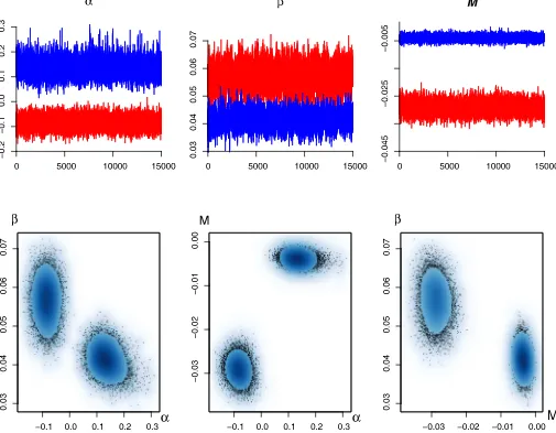
Figure 2. NUTS2 GDP growth data. Traces and scatterplots of the sampler forα,β, andM, usingK=2. Different shades indicate cluster assignment after postprocessing.
for each region. This means thatβnow corresponds to the aver-age long-run modal growth levels over time, whereasMcan be interpreted in terms of a stabilizing temporal effect. In partic-ular, for our situation with positive growth, negative values for μjwould imply a decreasing trend of growth over time within clusterj.
Figure2shows traces and scatterplots (with a smoothed den-sity representation) of the drawn values for (α,β,M)in the chain with two components
A second important conclusion that we can draw from Fig-ure2is that posterior dependence between the various cluster-specific parameters is quite small. This suggests that the pa-rameterization used clearly distinguishes between different as-pects of the data and that the parameters have a well-defined role.
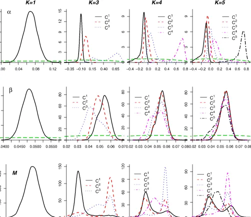
Figure3shows estimated marginal posterior densities for the model-specific parameters of the models with K=1,3,4,5. The graphs also plot the prior density, indicated by long dashes. Estimation of the common parameters is virtually unaffected by the number of clusters; Comparing the plots forαwith differ-entK’s clearly demonstrates the effect of pooling when units are not homogeneous; the pooled model (K=1) averages over
the whole panel, yielding misleading inference on the dynamics and an illusion of precise estimation (note the different scales). Moreover, it is clear from the inference on α withK=3,4, and 5 that these models contain more clusters than are sup-ported by the data, because there is no clear separation be-tween the clusters with lowerαj. This lack of separation leads to markedly multimodal posteriors forμjand clearly cannot be solved by choosing a different ordering constraint. It is reassur-ing that model choice through Bayes factors strongly avoids the inclusion of unwarranted clusters in our model. This illustrates in particular the sensible calibration of our prior assumptions.
As we noted in Table2, the two-cluster model is decisively preferred over the others. Posterior results are displayed in Fig-ure4. Note that the prior onλis improper, and thus its scaling is arbitrary. For this best model with two clusters, convergence is fairly rapid (values ofαjare not large in absolute value), and we have a small club of regions with small negative first-order growth autocorrelation (i.e., those with a small negative value of α) and a larger subset with small positive first-order auto-correlation, as indicated in the top left graph of Figure4. The posterior mean relative cluster sizes are{0.28,0.72}. In addi-tion, Figure5 shows the individual membership probabilities
Figure 3. NUTS2 GDP growth data. Prior (light long dashes) and posterior (as in legend) densities for the cluster-specific parameters, using
K=1,3,4,5. Different values ofKcorrespond to different columns. Rows relate to the densities ofα(top),β(middle), andM(bottom).Ci
indicates clusteri.
with the regions ordered in ascending order according to initial GDP level. This illustrates that the first cluster tends to con-sist of regions with relatively low GDP in 1995. In particular, it groups emerging regions (e.g., all of the Polish regions in the sample and most of the Czech regions) but also includes, for
Table 2. NUTS2 GDP growth data: Log BF, according to the number of clusters
K
K 2 3 4 5
1 −35 532 2037 2295
2 567 2071 2331
3 1504 1764
4 259
NOTE: A positive figure indicates support in favor of the model in the row.
example, inner London and Stockholm with high probability, which experience a similar, somewhat erratic, growth pattern (see Figure6in the sequel).
The first club has a meanα1value of−0.084, with (−0.130,
−0.038) the posterior CI of probability 0.95. For the other club, α2 has a mean value of 0.135 and lies within (0.073, 0.208) with a posterior probability of 0.95. Note that the posterior distribution of α for the pooled model (K =1) in Figure 3
is concentrated around an area that receives only very little probability mass from the posteriors ofα1 andα2 in the two-component model, so its averaged nature really does not cor-respond to any “observed” dynamic behavior. A summary of the marginal posterior distributions of βj, shown in Table 3, suggests that both clubs have different long-run average growth rates. The log Savage–Dickey density ratio in favor ofβ1=β2 is−17.3, strongly supporting a different average steady-state level. The economies with alternating growth dynamics (first
Figure 4. NUTS2 GDP growth data. Prior (long dashes) and posterior (as in the legend) densities for parameters of the model withK=2. For the cluster-specific parameters,Ciindicates clusteri.
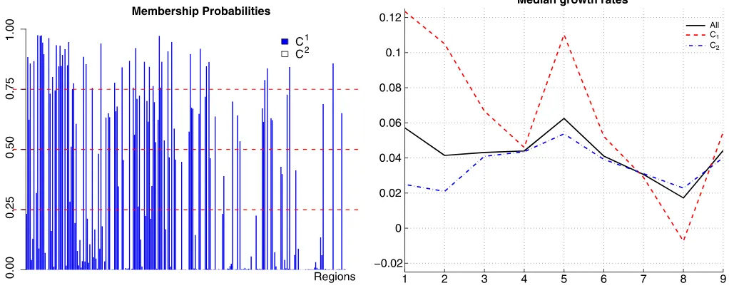
Figure 5. NUTS2 GDP growth data. Membership probabilities for the model withK=2, with the 258 units (regions) ordered according to initial GDP level. Bars indicate the posterior probability of belonging to cluster 1 for each region.
Figure 6. NUTS2 GDP growth data. Median observed GDP growth over countries with membership according to maximum posterior prob-ability. Solid line, full sample; dashed line, cluster 1; dot-dashed line, cluster 2.
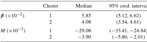
Table 3. NUTS2 GDP growth data. Summary statistics of
cluster) correspond to a higher median growth rate of around 5.9%, whereas the second group has a median of about 4.1%. The lower part of Table3presents the posterior estimates for the coefficients, µ. For the regions in cluster 1, μ1 tends to take large negative values, implying a fairly substantial negative trend of growth over time. For the second cluster, this effect is much smaller. Indeed, looking at Figure6, which groups aver-age (over regions) observed growth rates for each year, growth rates for cluster 1 clearly tend to decrease over the sample pe-riod, whereas those for cluster 2 remain almost unaffected. It also is apparent that the time pattern of growth rates for cluster 2 is more stable, with the negative value ofα1reflected in a more unstable growth pattern for cluster 1. This is in line with clus-ter 1 grouping mostly emerging economies, which are growing more rapidly in the beginning of the sample period. Interest-ingly, Figure6suggests convergence in growth between the two clusters by the end of the sample period.
Figure 4 illustrates that fat tails are a very prominent fea-ture of these data. Posterior inference onνis quite concentrated on small values in all cases, typicallyν∈(1.9,2.5)with 0.95 posterior probability. Some right skewness also is present in this data set. Indeed,γ∈(0.99,1.16)with posterior probability 0.95. However, the log Savage–Dickey density ratio in favor of γ=1 is 1.7, providing mild evidence in favor of the symmetric model.
Given this moderate evidence in favor of γ =1, we esti-mated the symmetric t model with K=2. The estimates of the common parameters and cluster membership probabilities (not shown) were little affected by imposing symmetry. We did, however, find some small differences for the cluster specific pa-rameters, which we present in Table4. Clearly, the symmetric model shifts the distribution of the long-run average levels β
to the right, to compensate for the right skewness in the data. Nevertheless, all estimated medians for the parameters of this model are contained in the corresponding 95% CIs of the skew version and vice versa.
Frühwirth-Schnatter and Kaufmann (2008) used a related setting to model the level of per capita income for a similar data
Table 4. NUTS2 GDP growth data. Summary statistics of the cluster-specific parameters, using the symmetrictmodel withK=2
Cluster Median 95% cred. interval
Table 5. NUTS2 income-level data. Summary statistics of the cluster-specific parameters using bothtmodels withK=2.
Values are median (95% CI)
set consisting of 144 regions for the 1980–1992 period. How-ever, the income data are scaled, for each time point, by the European average (see Canova2004). This effectively reduces the dynamic behavior of the individual regions to movement within the European distribution of incomes. In addition, this data set differs from our growth data in that it does not include any central European regions (or regions in Finland, Sweden, and Latvia). Bearing this in mind, we analyzed this data set chiefly for comparison with their results. We fitted our model to these level data, usingK=2 and no covariates. Like Frühwirth-Schnatter and Kaufmann (2008), we found two well-separated clusters, summarized in Table5, with estimated relative sizes
η=(0.13,0.87)′. Thus we have one small converged cluster withα1close to 0 and a large group with important dynamic behavior, whereα2is very close to 1. Despite the large differ-ences in dynamic behavior, there is no overwhelming difference in long-term levels (as measured byβ).
Clustering regions according to maximum posterior proba-bilities yields m1=15 and m2=129, not unlike the results
of Frühwirth-Schnatter and Kaufmann (2008). However, our membership assignments are not quite the same as those of Frühwirth-Schnatter and Kaufmann (2008). We must keep in mind, however, that their model uses initial income as a covari-ate for the membership probability.
Our model here differs from that used by Frühwirth-Schnatter and Kaufmann (2008) in a number of respects, some of which can have most effect on the results in this application, as fol-lows:
(i) We do not allow for unit roots, which is of some impor-tance here, because the AR(1) process on the levels is close to a unit root for one of the two clusters that they found (see their table 5 and our Table5). Note that with these data, we are modeling levels rather than growth rates.
(ii) The other priors also are quite different. They used nor-mals throughout, centered at 0 and with higher variances than ours. As we know, this will affect posterior odds between models.
(iii) They did not allow for skewness; however, left skewness is a prominent feature of the data, asγ∈(0.815,0.892) with probability 0.95. As we have seen with both the simulated data and the growth data, neglecting skewness can have a significant impact on the estimation of the steady-state levels.
(iv) They fixed the degrees of freedom for the Student t model at 8. In contrast, we find the tails to be ex-tremely fat, with(1.1,1.3)the 95% CI forν, regardless of the model used (skewed or symmetric). Of course,
this also will affect the estimated observational variance and might influence the clustering (see Sec.4.1).
In line with the latter point, the evidence favoring Student t tails over normal tails is overwhelming for both symmetric and skewed models. Once we choose a Student model, skew-ness is strongly preferred by the data. For normal models, how-ever, the log Savage–Dickey density ratio in favor ofγ =1 is 3.12, which is in line with the BF obtained from the bridge sampler. It is quite unusual to see the evidence favoring skew-ness disappear when we ignore the heavy tails. Thus, if we did not consider (unknown) heavy tails, we would be led dramati-cally astray in the evidence regarding skewness. Of course, all other models are massively dominated by the skew-tmodel. Ta-ble5presents the estimated cluster-specific parameters for both skewed and symmetrictmodels. The effect of neglecting skew-ness is similar to that with the previous data; whereas the dy-namics are little influenced by the inclusion of skewness, long-run levels are affected (but due to the left skewness, now in the other direction). Note thatβ2is shifted much more thanβ1.
5.2 Spanish Firm Employment
The data set was described in the appendix of Alonso-Borrego and Arellano (1999) and also used in Arellano (2003, sec. 6.7). It consists of a balanced panel of 738 manufacturing companies, recorded yearly from 1983 to 1990, and represents >40% of the Spanish value added in manufacturing in 1985.
In particular, we model employment growth in these firms. With our model described in Section2, and lettingK=1, we obtain 95% CIs of (0.04, 0.08) for α and (−0.0043, 0.0030) forβ. Again, inference on parameters common to models with different values ofKis virtually unaffected by the choice of the number of clusters.
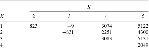
As shown in Table6,K=1 is strongly preferred overK=2, K=4 andK=5. But the model with three clusters performs considerably better than the pooled model, and we will concen-trate on the model withK=3 in the sequel. Because the model with five clusters was not preferred over any other model, we did not use larger values ofK.
Scatterplot of the drawn values for(α,β)in the chain with K=3, clearly suggesting that identifying the labels by ordering the values ofαjis the natural approach, just like in the previous example.
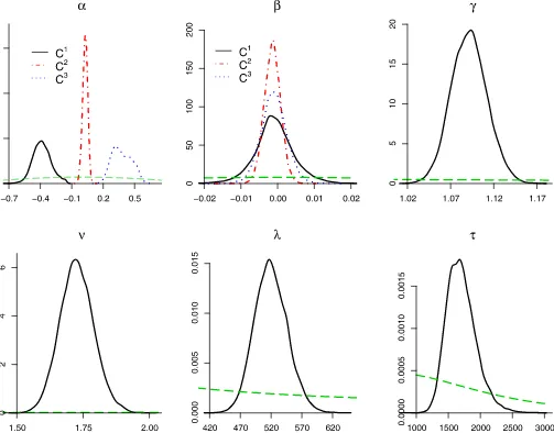
From the posterior densities in Figure7, it is apparent that tail behavior is extremely heavy and well determined by this (fairly large) data set. These data also clearly show right skewness with 95% CI (1.05, 1.13) forγ. Both the Savage–Dickey density
Table 6. Spanish firm data: Log BF, according to the number of clusters
NOTE: A positive number indicates support in favor of the model in the row.
ratio and bridge sampling indicate massive evidence in favor of the skewed model.
The relative size of each cluster (i.e., the average probability of cluster membership) is {0.132, 0.651, 0.217}.
We previously reported that the skewed model is strongly favoured by the data over its symmetric counterpart. To evaluate whether allowing for skewness makes a practical difference in this example, we have estimated the symmetric Student model (i.e.,γ=1) with three components. The main difference is in the equilibrium values βj. The posterior medians for βj with skewness are all within (−0.0011, −0.0008) and are now all positive, equal to {0.0057, 0.0051, 0.0058}, with the 95% CI for β2entirely on the positive real line. Thus, without taking into account the skewness, we would erroneously conclude that long-run employment growth is positive, whereas our skewed model assigns most probability to negative equilibrium growth of employment in Spanish manufacturing firms.
For both the skewed and symmetric cases, the three clusters of firms converge to very similar equilibrium levels, suggesting that we also might pool this parameter to gain strength. Fig-ure8 shows that the posterior density of the correlation para-meter a, as defined in (18), has a lot of mass close to 1 and thus strongly supports this model simplification. This is con-firmed by the formal log BF in favor of common βj’s, which is estimated at 13.4. Other parameters are virtually unaffected by this reduction of the model. The common long-run levelβ is (−0.005, 0.003) with posterior probability 0.95, very much in line with the results for cluster-specificβj’s with the skew-t model (see Figure 7), except that inference is now a bit more precise as a consequence of borrowing strength.
Finally, we calculate the predictive distribution of employ-ment in two firms in the sample for 1991 (1 year after the last observation in the sample), using a commonβ. Because we are predicting employment itself (rather than its growth), we condi-tion on the actual employment values in the sample years. Firms 433 and 31 are selected. The former grew from 30 to 37 em-ployees in 1990, and in the model withK=3, it is assigned to the three clusters with posterior weights{0.834,0.165,0.001}; the latter decreased its employment from 126 to 62 in 1990 and had cluster probabilities {0.324, 0.636, 0.040}. Figure 9
presents these predictives for the pooled model (K=1) and the model with three components (a symmetric version and a skewed version). The model withK=1 has a slightly positive αand thus will concentrate the predictive at a value that slightly extends the last observed movement. In the three-cluster model, firm 433 [Figure9(a)] has most mass on the first cluster, which corresponds to large negative values for α(see Figure7), and thus will counteract the last movement, resulting in much more predictive mass on lower employment values. Firm 31 has non-negligible mass for all three clusters, which results in a mul-timodal predictive, with the first cluster providing predictive mass around 80 (partially counteracting the last movement), and the third (least important) cluster resulting in slightly more weight on lower values. The latter is a consequence of the large positive values for the dynamics parameters, which lead to a pronounced extrapolation of the last observed change. Fi-nally, the second cluster (which has most of the weight) cor-responds to very small, mostly positive, values forα(see Fig-ure 7), which is translated in the large central mode, close to
Figure 7. Spanish firm data. Prior (long dashes) and posterior (as in legend) densities for parameters of the model with K=3. For the cluster-specific parameters,Ciindicates clusteri.
Figure 8. Spanish firm data. Posterior (solid) and prior (dashed) densities forain (18) usingK=3. Note thata∈(−1/(K−1),1).
Figure 9. Spanish firm data. Predictive distribution for 1991 for the employment of firms 433 (a) and 31 (b). Predictives are forK=1 (dashed) andK=3 (solid for skewed model, dotted for symmetric model). Employment numbers for 1989 and 1990 are indicated by dot-ted and solid vertical lines.
the last observed value (with a slight extrapolation of the last movement). The clusters vary mostly in terms of the dynam-ics parameter, so if the observed change is substantial (as is the case for firm 31), then multimodality in the predictive is easily generated. It is clear that the pooled model substantially underestimates the predictive uncertainty and can lead to dra-matically different conclusions. Of course, the different firms also have different individual effectsβi, but the effect of those on the one-step-ahead predictives shown is dominated by the dynamics. In the three-component model,β433 has a posterior
mean of 0.011 (corresponding to 1% growth), and the mean of β31 is−0.025. When we use the symmetric three-component
model (γ=1), the posterior means of these long-run levels are changed to 0.026 and−0.018, respectively, which constitutes a rather different picture for the equilibrium situation, especially for firm 433. Of course, this would affect the predictives for long forecast horizons, but short-run forecasting with the sym-metric model is not very different from that with the skewed model, as illustrated in Figure9.
6. CONCLUSION
In this article we have dealt with model-based clustering of longitudinal data, where the clusters can differ in dynamic and long-run equilibrium behavior, as well as in the effect of covari-ates on the equilibrium levels. We adopt flexible error distrib-utions, allowing for fat tails and skewness, each controlled by a single (easily interpretable) parameter. Prior distributions are carefully chosen to reflect a (commonly encountered) situation without strong prior information. Hierarchical prior structures are used to increase the robustness of our posterior results with respect to prior assumptions. The proposed prior structure gives the applied user the opportunity to conduct inference with these models without expending much effort on prior elicitation. We have provided a practically useful and very mild condition for the existence of the posterior distribution. We have used a sim-ple scatterplot of the drawn values for the cluster-specific para-meters to deal with the labelling problem.
Using simulated data, we assessed the ability of the model to distinguish between clusters and found that misspecifying the error distribution (by ignoring either skewness or fat tails) can negatively affect this clustering performance.
We analyze two real (balanced) panel data sets, one on per capita GDP growth of European regions, with 258 units and T =9, and one concerning employment growth in an even larger sample of 738 manufacturing firms withT=7. Both ap-plications favor clustering, ignoring the clustering in the data would result in totally misleading inference of the dynamic be-havior, parameterized byα; the pooled model averages out the dynamic behavior and does not properly account for the uncer-tainty. In both examples, the pooled posterior distribution forα is far too sharp, inducing a false sense of security. The effect of this is perhaps best appreciated by considering the predictive distribution. The shape, location, and concentration of the latter often are very different for the pooled model, as illustrated here for the firm data. In both applications skewness is important, not just statistically, but also in terms of the conclusions that we can draw from the data, as in, for instance, the firms example, where equilibrium growth levels are quite different if we ignore
the skewness, in that they would point to overall long-run em-ployment growth rather than to contraction.
It would be straightforward to extend the model to let the assignment of observations to clusters depend on covariates. A probit or logit specification (as in Frühwirth-Schnatter2004) would simply add one step to the MCMC sampler. In view of our discussion of the Spanish firm employment example, it would be natural to use firm size as a determinant of cluster probabilities in that case.
Other models for dealing with large numbers of time series have been proposed in the literature. For example, dynamic factor models as in Stock and Watson (2002) and Forni et al. (2005) are an alternative way to induce dimension reduction, especially when used in the context of macroeconomic fore-casting.
ACKNOWLEDGMENTS
This research was supported by EPSRC Grant GR/T17908/ 01. We gratefully acknowledge useful comments by one of the editors, an associate editor, two referees, and Eduardo Ley.
[Received June 2007. Revised December 2007.]
REFERENCES
Alonso-Borrego, C., and Arellano, M. (1999), “Symmetrically Normalised In-strumental Variable Estimation Using Panel Data,”Journal of Business & Economic Statistics, 17, 36–49. [63]
Arellano, M. (2003),Panel Data Econometrics, Oxford: Oxford University Press. [58,63]
Azzalini, A., and Capitanio, A. (2003), “Distributions Generated by Perturba-tions of Symmetry With Emphasis on a Multivariate Skew-tDistribution,” Journal of the Royal Statistical Society, Ser. B, 65, 367–389. [53] Baltagi, B. (2001),Econometric Analysis of Panel Data(2nd ed.), Chichester:
Wiley. [52]
Banfield, J. D., and Raftery, A. E. (1993), “Model-Based Gaussian and Non-Gaussian Clustering,”Biometrics, 49, 803–821. [52]
Bauwens, L., and Rombouts, J. V. K. (2007), “Bayesian Clustering of Many GARCH Models,”Econometric Reviews, 26, 365–386. [52]
Bensmail, H., Celeux, G., Raftery, A. E., and Robert, C. P. (1997), “Inference in Model-Based Cluster Analysis,”Statistics and Computing, 7, 1–10. [56] Berger, J. O., and Bernardo, J. M. (1992), “Ordered Group Reference Priors With Application to the Multinomial Problem,”Biometrika, 79, 25–37. [54] Canova, F. (2004), “Testing for Convergence Clubs in Income per capita: A Predictive Density Approach,”International Economic Review, 45, 49– 77. [53,58,62]
Casella, G., Mengersen, K. L., Robert, C. P., and Titterington, D. M. (2002), “Perfect Samplers for Mixtures of Distributions,”Journal of the Royal Sta-tistical Society, Ser. B, 64, 777–790. [56]
Casella, G., Robert, C. P., and Wells, M. T. (2004), “Mixture Models, Latent Variables and Partitioned Important Sampling,”Statistical Methodology, 1, 1–18. [56]
Celeux, G., Hurn, M., and Robert, C. P. (2000), “Computational and Inferential Difficulties With Mixture Posterior Distributions,”Journal of the American Statistical Association, 95, 957–970. [56]
Chib, S. (1995), “Marginal Likelihood From the Gibbs Output,”Journal of the American Statistical Association, 90, 1313–1321. [56]
Deschamps, P. J. (2006), “A Flexible Prior Distribution for Markov Switch-ing Autoregressions With Student-tErrors,”Journal of Econometrics, 133, 153–190. [55]
DiCiccio, J., Kass, R. E., Raftery, A. E., and Wasserman, L. (1997), “Comput-ing Bayes Factors by Combin“Comput-ing Simulations and Asymptotic Approxima-tions,”Journal of the American Statistical Association, 92, 903–915. [56] Diebolt, J., and Robert, C. P. (1994), “Estimation of Finite Mixture
Distribu-tions Through Bayesian Sampling,”Journal of the Royal Statistical Society, Ser. B, 56, 363–375. [55,56]
Diggle, P. J., Heagerty, P., Liand, K. Y., and Zeger, S. L. (2002),Analysis of Longitudinal Data(2nd ed.), Oxford: Oxford University Press. [52]