Full Terms & Conditions of access and use can be found at
http://www.tandfonline.com/action/journalInformation?journalCode=ubes20
Download by: [Universitas Maritim Raja Ali Haji] Date: 13 January 2016, At: 00:26
Journal of Business & Economic Statistics
ISSN: 0735-0015 (Print) 1537-2707 (Online) Journal homepage: http://www.tandfonline.com/loi/ubes20
Estimation and Welfare Analysis With Large
Demand Systems
Roger H von Haefen, Daniel J Phaneuf & George R Parsons
To cite this article: Roger H von Haefen, Daniel J Phaneuf & George R Parsons (2004)
Estimation and Welfare Analysis With Large Demand Systems, Journal of Business & Economic Statistics, 22:2, 194-205, DOI: 10.1198/073500104000000082
To link to this article: http://dx.doi.org/10.1198/073500104000000082
View supplementary material
Published online: 01 Jan 2012.
Submit your article to this journal
Article views: 87
View related articles
Estimation and Welfare Analysis With
Large Demand Systems
Roger H.
VONH
AEFENDepartment of Agricultural and Resource Economics, University of Arizona, Tucson, AZ 85721 (rogervh@ag.arizona.edu)
Daniel J. P
HANEUFDepartment of Agricultural and Resource Economics, North Carolina State University, Raleigh, NC 27695 (dan_phaneuf@ncsu.edu)
George R. P
ARSONSCollege of Marine Studies and Department of Economics, University of Delaware, Newark, DE 19716 (gparsons@udel.edu)
We develop an approach for estimating individual or household level preferences for a large set of quality-differentiated goods and for constructing Hicksian welfare measures within the demand system framework. Our approach uses a maximum simulated likelihood procedure to recover estimates of the structural parameters and a multistage, Monte Carlo Markov chain algorithm for constructing Hicksian consumer surplus estimates. We illustrate our approach with a recreation dataset consisting of day trips to 62 Mid-Atlantic beaches.
KEY WORDS: Beach recreation; Demand system models; Random parameters; Simulation; Welfare analysis.
1. INTRODUCTION
In this article we develop a demand system approach for estimating preferences for a large set of quality-differentiated goods at the individual or household level. We apply the ap-proach to an outdoor recreation dataset consisting of day trips to 62 beaches in the Mid-Atlantic region and analyze the wel-fare effects of changes in beach characteristics and availabil-ity. Interest in the value of beach recreation opportunities arises from policymakers’ need to assess the merits of beach nour-ishment programs and to measure the damages resulting from acute environmental accidents that impact beach availability. The Hicksian consumer surplus estimates reported in this arti-cle address these issues and represent the rst welfare measures derived from a theoretically consistent demand system model that accounts for interior and corner solutions and accommo-dates a large set of quality-differentiated goods.
Because of the computational difculties associated with estimating and generating welfare measures from demand system models, nearly all empirical strategies for modeling consumer choice for many goods have relied on the discrete choice random utility maximization (RUM) model developed by McFadden (1974). A large and growing body of empirical research has shown that the discrete choice RUM framework is attractive for modeling extensive margin choices made on single choice occasions, but how the framework can be mod-ied or augmented to represent consumer choices made over longer time horizons when realized demands are a mixture of interior and corner solutions remains an unresolved modeling issue. At present there are several discrete choice RUM-based approaches for modeling consumer choices in these situations (e.g., Morey, Rowe, and Watson 1993; Feather, Hellerstein, and Tomasi 1995; Hausman, Leonard, and McFadden 1995; Parsons and Kealy 1995), all of which have strengths and weak-nesses. Some common features of these RUM-based modeling
strategies are the assumptions that the time horizon of choice can be decomposed into separable choice occasions, that the ob-jects of choice on each choice occasion are quality-adjustedper-fect substitutes, and, with rare exception,that income efquality-adjustedper-fects are absent (for a more extensive review and comparison of these ap-proaches, see Parsons, Jakus, and Tomasi 1999). In part because of the restrictiveness of these assumptions, Phaneuf, Kling, and Herriges (2000; hereafter PKH) and Phaneuf (1999) reconsid-ered modeling consumer choice in these situations within a uni-ed demand system framework that consistently accounts for interior and corner solutions. Their empirical applications,how-ever, considered only a small number of quality-differentiated goods, and, thus, the relevance of the demand system frame-work for policy applications with many goods remained uncer-tain.
We demonstrate in this article that if preferences are ad-ditively separable the demand system framework can be es-timated and used to generate Hicksian welfare measures for applications with many goods. Additive separability implies strong restrictions for consumer behavior, but in our view these restrictions have similarities with the assumptions embedded in the discrete choice RUM models that have traditionally been used for this class of problems. Although discrete choice RUM models can generate substitution patterns that are more ex-ible than our additively separable demand system model, our model has the advantage of allowing for diminishing mar-ginal utility in consumption for a given commodity and, more generally, combining the intensive and extensive margins of consumer choice for all quality-differentiated goods in a coor-dinated and behaviorally consistent framework.
© 2004 American Statistical Association Journal of Business & Economic Statistics April 2004, Vol. 22, No. 2 DOI 10.1198/073500104000000082 194
In addition to permitting the construction of welfare mea-sures for a large set of quality-differentiated goods, our em-pirical models incorporate several innovations over existing demand system recreation applications. Our specications al-low a subset of the parameters entering the direct utility func-tion to vary randomly across individuals in the populafunc-tion. From an econometric perspective introducing random para-meters is attractive because it facilitates a relatively exible specication for the unobserved heterogeneity without substan-tially expanding the number of estimable parameters. In ad-dition, our empirical application incorporates an approach to welfare measurement suggested by von Haefen (2003) that con-ditions on an individual’s observed choice. In contrast to tradi-tional approaches to welfare measurement from RUM models (e.g., Small and Rosen 1981), we construct welfare measures in this article by simulating the unobserved heterogeneity enter-ing preferences such that our model predicts observed behavior perfectly at baseline conditions. The structure of the model is then used to predict how individuals respond to price, quality, and income changes. To implement our conditional approach, we develop a sequential Monte Carlo procedure that employs an adaptive Metropolis–Hastings algorithm. Whereas conditioning on an individual’s observed choice adds more complexity to our welfare calculation procedure, it substantially reduces the num-ber of simulations necessary to generate precise welfare esti-mates as well as the computational time involved.
Although our modeling approach can be applied to disaggre-gate consumption data for any number of quality-differentiated goods (e.g., transportation mode, brand level demand for com-modities such as cereal or coffee) and policy applications (welfare measurement, exact price index construction, valuing new goods), we illustrate its usefulness by assessing the wel-fare implications arising from changes in the availability and quality of outdoor recreation sites. Using a detailed dataset con-sisting of 540 Delaware residents’ beach recreation activities, our empirical application examines the demand for day trips to 62 ocean beaches in the Mid-Atlantic region. Owing to infre-quent but acute oil and toxic spills, state ofcials in New Jersey, Delaware, Maryland, and Virginia occasionally close beaches for health and safety reasons. In addition, beach erosion re-sulting from rising sea levels, development, and natural causes has led state ofcials to initiate beach nourishment programs throughout the region. Because beach recreators are among the individuals most affected by beach closures and erosion, our welfare scenarios can inform state ofcials of the potential eco-nomic losses arising from these impacts.
The remaining structure of the article is as follows. The next section gives a general overview of the issues involved in demand system estimation and welfare calculation with large choice sets. Section 3 follows with a discussion of the empir-ical specications and estimation strategies we employ in this article, and Section 4 discusses our strategy for constructing welfare measures. Section 5 discusses the Mid-Atlantic beach recreation dataset we use in our application, and Section 6 sum-marizes our estimation results. Section 7 discusses our welfare scenarios and results, and Section 8 concludes.
2. GENERAL OVERVIEW
In principle, there are two generic strategies for developing demand system models that consistently account for both inte-rior and corner solutions and can be applied to problems with many goods. The rst, developed independently by Hanemann (1978) and Wales and Woodland (1983) and referred to as the Kuhn–Tucker framework, exploits the Kuhn–Tucker conditions that implicitly dene the consumer’s optimal consumption bun-dle. Alternatively, Lee and Pitt (1986) developed a demand sys-tem framework that relies on the concepts of notional demand and virtual price functions (Neary and Roberts 1980). Although these approaches are dual, we focus on the Kuhn–Tucker frame-work in this section and in our subsequent empirical frame-work. Much of our general discussion that follows, however, transfers to the dual approach in a straightforward manner.
As discussed in, for example, PKH, the Kuhn–Tucker frame-work begins with a specication of consumer preferences repre-sented by a continuously differentiable, strictly increasing, and strictly quasi-concave direct utility function,U.x;Q;z;¯;"/, where x is an M-dimensional vector of consumption lev-els for the quality-differentiated goods that are consumed in nonnegative quantities, Q denotes an M £K matrix of commodity-specic quality attributes of the goods in x (i.e., QD[q1; : : : ;qM]T, whereqi;iD1; : : : ;M, is aK£1 vector of
attributes for goodi),zis an essential Hicksian composite com-modity representing spending on all other goods,¯is a vector of structural parameters entering preferences, and" is a vector or matrix of unobserved heterogeneity.Because"is interpreted as components of the utility function known by the individual but unobserved and random from the analyst’s perspective, the structure of preferences is consistent with McFadden’s random utility maximization (RUM) hypothesis (see McFadden 2001 for a recent discussion).
The consumer maximizes utility subject to a linear budget constraint andMnonnegativityconstraints:
max
x;z U.x;Q;z;¯;"/ s:t: p
TxCzDy;x¸0; (1) wherepis anM-dimensional vector of prices, yis income, and the price of the Hicksian composite commodity is normalized to 1 with no loss in generality. In addition to the constraints in (1), the Kuhn–Tucker conditions that implicitly dene the optimal solution to the consumer’s problem can be written as
@U=@xj·.@U=@z/pj; jD1; : : : ;M; (2)
xj¡@U=@xj¡.@U=@z/pj¢D0; jD1; : : : ;M: (3)
Estimation of the structural parameters entering the preference specication within the Kuhn–Tucker framework exploits (2). These weak inequalities and an individual’s observed choices place restrictions on the support of the unobserved heterogene-ity’s distribution. Assuming the errors representing unobserved heterogeneity are drawn from some known family of distribu-tions with parameter vector6, these restrictions permit recov-ery of estimates for¯ and6 within the maximum likelihood framework.
From an econometric perspective the Kuhn–Tucker model can be interpreted as an endogenous regime-switching model
where regimes are dened as combinations of interior and cor-ner solutions for the M goods and determined by (2). When dealing with applications involving many goods, two related issues must be resolved in order to estimate Kuhn–Tucker en-dogenous regime-switching models. The analyst must choose a exible yet parsimoniously parameterized direct utility func-tion. This requires restricting the dimension of ¯ to be sufciently low. Moreover, the analyst must specify a distrib-ution for the unobserved heterogeneity that has an estimable parameter vector 6 that is of relatively low dimension and that allows calculation of the multiple-dimensional integrals that correspond to the probabilities of observing each of the 2M possible regimes. If these issues are adequately addressed, the Kuhn–Tucker demand system framework represents a vi-able approach for estimating consumer preferences for many quality-differentiated goods.
Welfare measurement from demand system models raises a separate and in many ways more complicated set of issues. The Hicksian consumer surplus,CSH, associated with a price and quality change from.p0;Q0/to.p1;Q1/is implicitly dened where!indexes each of the 2Mseparate regimes andV
!.¢/ rep-resents the corresponding conditional indirect utility function. Unless preferences are quasilinear or homothetic in income, no closed-form solution exists for CSH, and iterative techniques such as numerical bisection are required to solve forCSH. How-ever, as discussed by PKH, procedures such as numerical bi-section require that the analyst solve the consumer’s problem at each iteration conditional on an arbitrary set of.p;Q;y;"/ val-ues. PKH proposed a strategy for accomplishing this task that analytically calculates each of the possible 2M conditional in-direct utility functions and ascertains which is the maximum. Although this strategy is computationally feasible for smallM, it quickly becomes intractable asM grows large. For example, in our subsequent empirical application whereMequals 62, the number of possible regimes is 4:6117£1018.
An additional complication with constructing welfare esti-mates is that the analyst does not observe". This limitation suggests that the analyst cannot determine the individual’s Hicksian consumer surplus precisely and can at best construct an estimate of the welfare measure’s central tendency over the support of " such as its expectation,E.CSH/. As described in PKH constructingE.CSH/requires the use of Monte Carlo techniquesthat involve simulating several realizations of"from its estimated distribution, solving for CSHconditional on each simulated", and averaging the simulated values of CSH. In-creasing the number of simulations improves the precision of the estimate but also increases the computationaltime involved. One nal notable difculty arises because these welfare es-timates are functions of eses-timates of¯and6 that are random variables from the analyst’s perspective. Quantifying the im-plications of uncertainty about the parameters’ true values by constructing standard errors for the welfare estimates requires replication of the entire simulation routine for several alterna-tive parameter estimates.
The preceding discussion suggests the signicant compu-tation challenges arising with welfare estimation from de-mand system applications with large choice sets. For welfare measurement to be viable with demand system models, the analyst must be able to quickly solve for the utility the indi-vidual obtains conditional on.p;Q;y;"/. As discussed in the Introduction, the difculties associated with this task as well as estimating demand system models have led researchers in the outdoor recreation literature to largely abandon demand system models and instead rely on the discrete choice RUM frame-work. More recently, researchers in the eld of industrial or-ganization have also adopted the discrete choice framework for modeling this class of problems due to its computational ad-vantages (e.g., Berry, Levinsohn, and Pakes 1995; Nevo 2001). In the next section we develop econometrically tractable pref-erence specications that can be used to model the demand for a large set of quality-differentiated goods and to construct Hicksian welfare measures.
3. PREFERENCE SPECIFICATIONS AND ESTIMATION STRATEGIES
In this article our approach to modeling consumer choice within the Kuhn–Tucker demand system framework relies on the assumption that consumer preferences are additively sepa-rable in each element ofxandz:
where we have suppressed all arguments entering preferences exceptx and z in (5). This specication of preferences has similarities with the utility structures employed by Hanemann (1984) and Chiang and Lee (1992) to model mixed dis-crete/continuous choices. Their preference specications can be nested within the following general form:
U.x;z/Du
Note that the structure in (6) assumes that the elements ofx en-ter preferences additively through a separable subfunction and, therefore, are perfect (quality-adjusted) substitutes, although the elements of x collectively need not be additively separa-ble from z. By contrast, (5) implies that strictly increasing, strictly concave functions of each element ofxandzenter pref-erences additively.Hanemann’s and Chiang and Lee’s approach to structuring preferences implies that the individual consumes at most one element ofx, whereas our preference structure gives rise to multiple elements ofxbeing consumed.
Although PKH also assumed preferences are additively sep-arable in their empirical work, we recognize that it is a strong preference restriction; it rules out a priori inferior goods and implies that all goods are Hicksian substitutes (see Pollak and Wales 1992 for a discussion). Additive separability, moreover, implies that the marginal utility for each good is independent of the level of all other goods. Thus, although the preference function is consistent with the intuitively appealing notion of diminishing marginal utility of consumption for a given good, it does not allow marginal utility to decrease (or increase) with
increases in consumption of other goods. This in turn limits the richness of substitution patterns that can be captured with this preference structure.
For perspective, it is instructive to compare these implica-tions with those that arise from the separability assumpimplica-tions embedded in discrete choice RUM models. These models de-compose the time horizon of choice into separable choice occasions on which the individual makes discrete choices. Consumer behavior across each of the choice occasions is un-coordinated and, thus, diminishing marginal utility of consump-tion for a good is absent from these models. Although discrete choice RUM models can generate fairly rich substitution pat-terns among goods, they assume that on a given choice occasion all goods are quality-adjustedperfect substitutes and income ef-fects are absent (for a notable exception, see Herriges and Kling 1999).
The additively separable empirical demand system specica-tions estimated in this article can be nested within the following general structure:
wheresanddj are vectors of individual specic demographic
variables and site-specic dummy variables, respectively;µ D
[µ1; : : : ; µM]T>0I½D[½1; : : : ; ½M; ½z]<1I±;³, and ° are
estimable parameters; ("±;"³/ represent unobserved hetero-geneity that varies randomly across individuals in the popula-tion; and."1; : : : ; "M/represent unobserved heterogeneity that
varies randomly across individuals and goods.
Our preference structure is a close relative of the linear ex-penditure system employed by PKH but differs in three im-portant respects. First, our specication can be interpreted as a more general specication because, in the limit as all elements of½approach 0, our specication nests the linear expenditure system, that is,
Second, PKH assumed, using our notation in (7), that a good’s quality attributes enter preferences through9instead ofÁ. This approach to introducing quality implies that weak complemen-tarity (i.e.,@U=@qjD0 ifxjD0;8j; see Mäler 1974; Bradford
and Hildebrandt 1977 for discussions) is not, in general, satis-ed unlessµjD0 when½j6D0 andµjD1 for the limiting case
when½jD0;8j. As a result a potentially large component of
the total value associated with a quality change will be indepen-dent of the consumer’s use of a particular commodity, a concep-tually troubling implication for many applications. Because our specication introduces quality through the simple repackaging Áparameters (Griliches 1964), weak complementarity is satis-ed for all parameter values; thus, only use-related values will
arise from our model. Finally, our specication allows the para-meters for the demographic and site-specic dummy variables entering the9parameters to vary randomly across individuals in the population. As discussed later, this feature of our model allows us to introduce a more exible structure for unobserved heterogeneity.
Maximizing the utility function in (7) with respect topTxC
zDyand the nonnegativity constraints implies a set of rst-order conditions that, with some manipulation, can be written as These weak inequalities, along with assumptions for the dis-tributions of"D."±;"³; "1; : : : ; "M/, permit estimation of the
structural parameters using maximum likelihood techniques. In our application we assume that each"j is an independent and
identically distributed draw from the Type I extreme-value dis-tribution with common scale parameter¹. Dening the right side of (9) asgj."±;"³/, the likelihood of observing a particular
where J is the Jacobian of transformation. The unconditional likelihood of observingxis
l.x/D
Z
l.xj"±;"³/f."±;"³/d"±d"³; (11) where the integral is over the full support of ."±;"³/. For our application we assume that ."±;"³/ are mean-zero ran-dom draws from the normal distribution with unequal vectors of scale parameters (¾±;¾³/and no correlations. Given these as-sumptions and the structure of our conditional likelihood func-tion, (11) has no closed-form solution and cannot be evaluated using numerical integration techniques unless the dimension of."±;"³/is small. In this article, we follow common empirical practice in the discrete choice literature (e.g., Train 2003) and use simulation to evaluate (11). Our estimation strategy, there-fore, falls under the rubric of maximum simulated likelihood estimation (Gourieroux and Monfort 1996). Although estima-tion of our random parameter model is more computaestima-tionally difcult than the xed parameter model with generalized ex-treme value unobserved heterogeneity employed by PKH, it is more exible. In addition to allowing for heteroscedasticity and correlations in the unobserved heterogeneity across groups of goods as PKH’s specication does, our specication also allows for heteroscedasticity across individuals.
4. WELFARE CALCULATION
4.1 Solving the Consumer’s Problem
An essential component of constructing Hicksian welfare measures involves evaluating the utility an individual achieves conditional on.p;Q;y;"/. When the dimension of the choice set is large, PKH’s strategy of analytically constructing all 2M
possible conditional indirect utility functions and determining which is the maximum is not feasible. In this article, we pursue an alternative, computationally tractable strategy that numeri-cally solves the Kuhn–Tucker conditions for the optimal con-sumption levels. These optimal values are then inserted into the direct utility function to ascertain the individual’s utility condi-tional on.p;Q;y;"/.
Given our additive separability assumption, solving the con-sumer’s problem is greatly simplied. In particular, the Kuhn– Tucker conditions take the general form:
@uj.xj/
@xj
·@uz.z/
@z pj 8j; (12)
xj
µ@u
j.xj/
@xj
¡@uz.z/
@z pj
D0 8j; (13)
xj¸0 8j; (14)
zDy¡X
j
pjxj: (15)
Note that additive separability implies that only xj andz
en-ter thejth inequalities in (12)–(14). This structure suggests that if the analyst knew the optimal value for z, he or she could use (12)–(14) to solve for eachxj. Therefore, solving the
con-sumer’s problem reduces to solving for the optimal value ofz. Building on this insight, we developed the following numerical bisection algorithm to solve the consumer’s problem:
1. At iteration i set ziaD.zli¡1Cziu¡1/=2. To initialize the algorithm, setz0l D0 andz0uDy.
2. Conditional onzia, solve forxiusing (12)–(14). 3. Use (15) andxito constructQzi.
4. If zQi >zia set zil Dzia and ziu Dziu¡1. Otherwise, set
zilDzil¡1andziuDzia.
5. Iterate until abs.zil¡ziu/·c, wherecis arbitrarily small. The ability of our algorithm to solve the consumer’s prob-lem relies on the strict concavity of our utility function.note that monotonic transformations of the utility function will not affect the consistency of our algorithm). By totally dif-ferentiating (12), one can show that strict concavity implies @xj=@z¸0 8j. This inequality, in conjunction with the fact that
our model has a unique solution,.x¤;z¤/, suggests that ifziais less than or equal toz¤, the implied solutions for the quality dif-ferentiated goods,xi, will be less than or equal to their optimal solutions, and, by implication,Qzi¸zia. Conversely, ifzia¸z¤, each element ofxiwill be greater than or equal to its optimal so-lution, and, by implication,Qzi·zia. These relationships suggest that updating the upper and lower bounds using the criteria stip-ulated in step 4 and iterating will solve for.x¤;z¤/to any level of precision. Plugging these optimal solutions into (7) allows the analyst to evaluate the consumer’s utility conditional on (p;Q;y;"/. Nesting this algorithm for solving the consumer’s problem within a numerical bisection routine that iteratively solves for the income compensation that equates utility before and after the price and quality change will allow the analyst to construct the Hicksian consumer surplus,CSH.
Additional insight into how our algorithm for solving the consumer’s problem works is provided graphically in Figure 1.
Figure 1. Solving the Consumer’s Problem.
The real line from.0;y] represents the feasible set of values thatz¤ can take. For illustration assume that, unknown to the analyst,z¤ is located as shown in Figure 1. To initialize our numerical bisection algorithm, we set z0l D0 and z0hDy. At the rst iteration we insert the average ofz0l andz0h (i.e., z1a) into (12)–(14) to solve for the implied demands,x1. Using the budget constraint, we solve forzQ1. Becausez1ais less thanz¤, the curvature properties of (12) imply thatzQ1will be greater thanz1a, and, thus,z1acan be used to update the lower bound (z1l Dz1a). Keeping the upper bound estimate the same (z1uDz0u), this rou-tine can be iterated a second time where it is found thatz2a>zQ2. As a result the upper bound estimate is updated in the second iteration withz2a whereas the lower bound remains unchanged (i.e.,z2uDz2aandz2l Dz1l). This numerical bisection procedure can be used to solve for.x¤;z¤/to any level of precision by replicating these basic steps.
4.2 Efcient Simulation of the Unobserved Heterogeneity
The algorithm described in the previous section permits construction of welfare measures conditional on a set of unobserved heterogeneity values. As discussed in Section 2, a precise estimate of the individual’s Hicksian consumer sur-plus is not possible because the elements of"are not observed. However, using simulation techniques and the distribution of the unobserved heterogeneity, the analyst can construct esti-mates ofCSH such as its expectation,E.CSH/. The approach taken by PKH to simulating the unobserved heterogeneity em-ploys the full distributional support of". In this article, we build on an approach suggested by von Haefen (2003) and in-stead simulate the unobserved heterogeneity from the region of the unobserved heterogeneity’s support that is consistent with the individual’s observed choice. In other words, we simulate"
such that at baseline conditions our model perfectly predicts the observed choices we nd in our data, and we use the model’s structure of substitution to predict how individuals respond to price, quality, and income changes. This approach contrasts with PKH’s more traditional approach that uses the structure of the model to predict both what individuals do at baseline conditions as well as how they respond to price, quality, and income changes. For the purposes of our application in this
article, incorporating observed choice is appealing because, al-though it requires the use of more complicated simulation tech-niques, it greatly reduces the number of simulations required to produce a precise estimate ofE.CSH/as well as the computa-tional time involved. Based on some Monte Carlo experiments with low-dimensional choice sets, we found that, relative to the unconditional approach, the conditional approach to welfare measurement required roughly one-third the simulations and time to produce mean welfare estimates that were insensitive to additional simulations.
We follow von Haefen and use a sequential strategy to simu-late the unobserved heterogeneity consistent with the individ-ual’s observed choice. Note that our objective is to simulate from the distribution of " conditional on x;f."jx/. This dis-tribution can be decomposed as follows:
f."jx/Df1."±;"³jx/f2."1; : : : ; "Mj"±;"³;x/: (16) Equation (16) states that the joint conditional distribution for the unobserved heterogeneity can be decomposed into the mar-ginal distribution for the random parameters conditional onx multiplied by the conditional distribution for the site-specic unobserved heterogeneity conditional onxand the random pa-rameters. We use an adaptive Metropolis–Hastings algorithm (Chib and Greenberg 1995) tailored to our problem to simulate fromf1."±;"³jx/. The steps of the algorithm are as follows:
1. At iterationi simulate a candidate vector of unobserved heterogeneity,."Qi±;"Qi³/, from the normal distribution with location parameters ."i±¡1;"i³¡1/ and scale parameters (ri¡1¾±;ri¡1¾³/ where ri¡1 is a constant. To initialize the process, set each element of."0±;"0³/equal to 0 and
r0equal to .1.
2. Construct the following statistic:
ÂiD N."Q
i
±=¾±;"Qi³=¾³/l.xj Q"i±;"Qi³/
N."i±¡1=¾±;"i³¡1=¾³/l.xj"±i¡1;"i³¡1/
; (17)
whereN.¢/is the probability density function for the nor-mal distribution and l.¢/ is dened in (10). If Âi ¸U
where U is a uniform random draw, accept the candidate random parameters, that is,."i±;"i³/D."Qi±;"Qi³/. Otherwise, set."i±;"i³/D."i±¡1;"i³¡1/.
3. Gelman, Carlin, Stern, and Rubin (1995) argued that the Metropolis–Hastings algorithm for the normal distribu-tion is most efcient if the acceptance rate of candidate parameters is between .23 and .44. Accordingly, we em-ploy the following updating rule for ri. If the propor-tion of accepted candidate parameters is less than .3, set
riD1:1ri¡1. Otherwise, setriD:9ri¡1. 4. Iterate.
After a burn-in period, this Monte Carlo Markov chain simu-lator generates draws fromf1."±;"³jx/that can be used to con-structE.CSH/.
After values of ."±;"³/ are simulated, drawing from
f2."1; : : : ; "Mj"±;"³;x/is far simpler. If goodj is consumed in a strictly positive quantity, the structure of our model, the simulated random parameters, and the individual’s observed choice imply that"jiDgj."i±;"i³/, wheregj.¢/is the right side
of (9). Otherwise,"jican be simulated from the truncated Type I extreme value distribution via
"ijD ¡ln¡¡ln¡exp¡¡exp.¡gj."i±;"i³/=¹/
¢
U¢¢¹; (18) whereUagain is a uniform random draw.
4.3 Summary
Before proceeding to the data summary and empirical results, we summarize the key components of our welfare measurement algorithm:
1. For simulationiuse the sequential procedure described in the previous section to simulate" consistent with the individual’s observed choice. Because simulating from
f1."±;"³jx/requires the use of an adaptive Metropolis– Hastings algorithm, discard the rstTsimulations. 2. For everyjth simulation after the rstT, use a numerical
bisection routine to solve for the simulated Hicksian con-sumer surplus associated with a price and quality change.
jis generally set to some value greater than 1 to reduce the impact of serial correlation in the Markov chain se-quence for."±;"³/.
2a. At each step of the numerical bisection routine that solves for the Hicksian consumer surplus associated with a given simulation, use the numerical bisection routine described in Section 4.1 to solve the consumer’s prob-lem. Inserting these optimal values into (7) permits the analyst to determine the utility the individual achieves. 3. Average each of the simulated Hicksian consumer
sur-plus values to construct an estimate ofE.CSH/, the indi-vidual’s expected Hicksian consumer surplus.
Although our algorithm for estimating welfare measures has multiple layers and numerous details, our experience has been that it is surprisingly easy and fast to use in an applied setting. One of the algorithm’s most appealing attributes is that each of its steps can be executed simultaneously for every observa-tion in the sample using vector and matrix notaobserva-tion. This fea-ture implies that coding and executing the algorithm in a matrix programming language reduces the computational burden sig-nicantly.
5. APPLICATION
We apply our demand system framework to a random sample of Delaware residents’ recreational day trips to Mid-Atlantic ocean beaches in 1997. From a policy perspective understand-ing beach recreation demand is important for at least two rea-sons. Oil and toxic spills in coastal waters often result in beach closings. Under the Oil Pollution Act of 1990 and other Natural Resource Damage Assessment (NRDA) statutes, the public’s lost economic benets arising from these spills are compensable. Deacon and Kolstad (2000) discussed issues as-sociated with estimating these losses and argued that revealed preference recreation demand models are a preferred method for ascertaining beach users’ resource values. Furthermore, un-derstanding how characteristics such as beach width inuence the demand for beach recreation can help inform the ongo-ing debate over beach nourishment as a strategy for combatongo-ing
coastal erosion. Beach nourishment, or pumping imported sand onto an eroding beach, is a technically feasible but costly en-gineering approach for maintaining coastal areas threatened by erosion from rising sea levels, development, and natural causes. At present, substantial state and federal resources have been earmarked for these activities in response to a perceived need to protect tourism and recreation-related infrastructure. The lit-erature reviews presented in Massey (2001) and Parsons and Massey (2003) suggest that environmental economists’ under-standing of the recreational values associated with policies that impact beach erosion and availability are in many ways incom-plete and outdated.
To assess the recreational values of beach amenities and to gauge residents’ willingness to pay for beach quality im-provements such as nourishment, researchers at the University of Delaware collected data on visits by Delaware residents to 62 ocean beaches in New Jersey, Delaware, Maryland, and Vir-ginia during 1997. Figure 2 shows a map of the region and several of the major beaches included in the dataset. Massey (2001) discussed the data collection effort in detail. A mail survey of 1;000 Delaware residents selected via stratied ran-dom sampling resulted in 540 completed responses. Although respondents provided information on the number of day trips, multiday trips, and side trips made to each of the 62 beaches, we follow conventional empirical practice in the recreation lit-erature and consider only day trips in our analysis. Excluding multiday and side trips from our analysis implies that our ag-gregate welfare estimates are incomplete measures of the total value of beach recreation. The exclusion does, however, allow
Figure 2. Mid-Atlantic Application Region.
us to avoid the difcult modeling issues arising when on-site time at a beach is a separate argument of the individual’s utility function and when recreation trips involve multiple activities and jointly produce multiple service ows. For further discus-sion of these and other important issues pertaining to recreation demand modeling, see Phaneuf and Smith (2003).
The survey collected sufcient information to compute round trip travel costs to each of the beaches. For every individual in the sample, a beach’s price is assumed to consist of transit costs (valued at $.35 per mile), beach fees, highway tolls, parking fees, a ferry toll on trips from southern Delaware to New Jersey beaches, and the opportunity cost of travel time valued at the individual’s average wage rate. Distances and travel times to each of the 62 sites from each of 540 residents’ homes were calculated using PC Miler. The wage rate was estimated as the individual’s annual income divided by 2;040 (i.e., the typical number of hours worked in a year).
Household characteristic and demographic data were also collected and are used to parameterize our utility function. Household-specic variables and recreational summary statis-tics are listed and described in the top part of Table 1. Note that respondents took on average 9.77 trips and visited 2.77 different beaches during the season. The maximum number of beaches visited by a respondent was 19, and 165 people sur-veyed (30% of the sample) did not visit any beaches during the season.
In addition to the behavioral data, auxiliary information on the characteristics of the 62 beaches was also gathered. Four-teen variables are used to differentiate the beaches included in the study. These variables are listed and described in the lower part of Table 1. Of interest for policy purposes are the indica-tor variables for wide and narrow beach. Of the 62 beaches, 25% are wide (i.e., greater than 200 feet in width) and 14% are narrow (less than 75 feet in width). The impacts of the wide and narrow dummy variables on the demand for beach visits allow us to gauge the effects of beach width on recreation demand and to assess the welfare implications of policies designed to alter beach width such as beach nourishment.
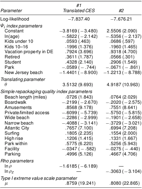
6. PARAMETER ESTIMATES
Although we estimated several demand system specica-tions consistent with the generic structure described in Sec-tion 3, we only present a representative set of our ndings in this section. Table 2 contains estimates for two xed pa-rameter models (i.e., "± D"& D0/ nested in (7): a trans-lated constant elasticity of substitution (CES) specication (column 2) resulting from the restrictions½zD½jD½ ; 8jand
µjDµ ;8j, and a second specication (column 3) resulting from
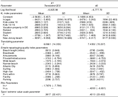
the restrictions½jD0; 8jandµjDµ ; 8j. Table 3 contains
es-timates for more general random parameter versions of these specications that allow the parameters in the9 index to vary randomly across the population. Although the parameter esti-mates in Table 2 are estimated with conventional maximum likelihood techniques, the parameter estimates in Table 3 are obtained via maximum simulated likelihoodprocedures. To im-prove simulation efciency, we follow common empirical prac-tice in the discrete choice literature and employ Halton draws rather than random draws in the calculation of our simulated
Table 1. Household and Beach Characteristics Variables
Variable Description Summarya
Household-specic variables
ln(age) Natural log of respondent age 3.82 (.33) Kids under 10 Respondent has kids under 10 (0/1) .26 Kids 10–16 Respondent has kids between 10 and 16 (0/1) .20 Vacation property in DE Respondent owns vacation home in DE (0/1) .03 Retired Respondent is retired (0/1) .24 Student Respondent is student (0/1) .05 Income Household annual income 49,944 (30,295) Trips Total visits for day trips to all sites 9.77 (14.06) Sites visited Number of beaches visited during 1997 2.70 (3.19)
Site characteristicsb
Beach length Length of beach in miles .62 (.87) Boardwalk Boardwalk with shops and attractions (0/1) .40 Amusements Amusement park near beach (0/1) .13 Private/limited access Access limited (0/1) .25 Park State or federal park or wildlife refuge (0/1) .09 Wide beach Beach is more than 200 feet wide (0/1) .25 Narrow beach Beach is less than 75 feet wide (0/1) .14 Atlantic City Atlantic City indicator (0/1) .016 Surng Recognized as good surng location (0/1) .35 High rise Highly developed beach front (0/1) .24 Park within Part of the beach is a park area (0/1) .14
Facility Bathrooms available (0/1) .48
Parking Public parking available (0/1) .45 New Jersey beach New Jersey beach indicator (0/1) .74 Price Person-specic money and time cost of travel $118c
a Summary statistics for household variables are means (standard errors) over the 540 individuals. Summary statistics for site variables are means (standard errors) over the 62 sites.
b We thank Tony Pratt and Michael Powell of the Department of Natural Resources and Environmental Control and Steve Hafner of the Coastal Research Center at Richard Stockton College of New Jersey for their help in compiling and verifying the characteristics data.
cThis statistic is the mean (standard error) of each individual’s mean trip price. Each individualin the sample has a unique price associated with visiting each of the 62 sites. Because prices are functions of distance, there is substantial variability in site prices both for and across individuals.
Table 2. Kuhn–Tucker Fixed Parameter Estimates¤
#1
Parameter Translated CES #2
Log-likelihood ¡7;837:40 ¡7;676:21
ªi index parameters
Constant ¡3:8169 (¡3:480) 2:5506 (2:090) ln(age) ¡:5822 (¡2:142) ¡:5356 (¡2:137) Kids under 10 :0593 (:463) :0686 (:597) Kids 10–16 :1996 (1:376) :1960 (1:465) Vacation property in DE :7924 (3:696) :9318 (4:700) Retired :3611 (1:787) :0566 (:301) Student :4328 (2:140) :2906 (1:549) Park ¡:0589 (¡:744) ¡:0671 (¡:861) New Jersey beach ¡1:4401 (¡8:900) ¡1:2213 (¡8:788)
Translating parameter
µ 3:5132 (9:693) 4:9187 (10:963)
Simple repackaging quality index parameters
Beach length (miles) :0726 (1:843) :0764 (2:029) Boardwalk ¡:2199 (¡2:670) ¡:2020 (¡2:575) Amusements :8568 (9:178) :7551 (8:641) Private/limited access ¡:6099 (¡5:739) ¡:5750 (¡5:815) Wide beach ¡:2286 (¡2:999) ¡:1901 (¡2:658) Narrow beach ¡:4088 (¡3:141) ¡:3729 (¡3:021) Atlantic City :7657 (7:100) :6994 (7:208) Surng :1805 (2:235) :1554 (2:000) High rise :1206 (1:415) :1331 (1:667) Park within :5775 (6:220) :5256 (5:943) Facility ¡:0347 (¡:582) ¡:0275 (¡:440) Parking :4996 (5:126) :4667 (4:706)
Rho parameters
ln½ ¡1:6185 (¡6:189) —
ln½z — ¡:3063 (¡3:104)
Type I extreme value scale parameter
¹ :8759 (19:241) :8080 (22:865)
¤t-statistics based on robust standard errors in parentheses.
Table 3. Kuhn–Tucker Random Parameter Estimates¤
#1
Parameter Translated CES #2
Log-likelihood ¡6,825.98 ¡6,777.70
ªi index parameters Mean SD Mean SD
Constant ¡2:5630 (¡5:457) — 3:1698 (4:453) — ln(age) ¡:6421 (¡5:800) :2396 (16:975) ¡:6478 (¡5:242) :1994 (22:493) Kids under 10 :0805 (1:137) :0107 (:142) :0588 (:818) :0306 (:609) Kids 10–16 :2688 (3:873) :1403 (2:734) :1189 (1:535) :0564 (1:082) Vacation property in DE :6985 (5:528) :3650 (6:264) :9131 (11:170) :0668 (4:119) Retired :2993 (3:725) :1034 (4:976) ¡:0031 (¡:034) :1534 (4:100) Student :2605 (2:664) :0746 (1:210) :3026 (3:505) :1210 (4:542) Park ¡:0758 (¡1:247) :3578 (7:462) ¡:0870 (¡1:469) :3416 (6:606) New Jersey beach ¡:9097 (¡9:058) :9890 (16:686) ¡:9747 (¡8:317) :9177 (9:550)
Translating parameter
µ 6.0661 (14.353) 7.4352 (15.237)
Simple repackaging quality index parameters
Beach length (miles) .0813 (3.648) .0795 (3.409)
Boardwalk ¡.0366 (¡.687) ¡.0540 (¡.999)
Amusements .5880 (9.146) .6007 (9.348)
Private/limited access ¡.3743 (¡6.794) ¡.3880 (¡6.753)
Wide beach ¡.1575 (¡3.195) ¡.1564 (¡3.072)
Narrow beach ¡.2343 (¡3.244) ¡.2428 (¡3.233)
Atlantic City .5115 (5.859) .5419 (5.979)
Surng .0983 (1.946) .1034 (1.991)
High rise ¡.0404 (¡.758) ¡.0247 (¡.452)
Park within .3718 (5.663) .3876 (5.787)
Facility ¡.0086 (¡.268) ¡.0123 (¡.340)
Parking .2396 (3.737) .2625 (4.011)
Rho Parameters
ln½ ¡1.7876 (¡7.798) —
ln½z — ¡.4200 (¡6.831)
Type I extreme value scale parameter
¹ .3817 (22.421) .4013 (23.432)
¤t-statistics based on robust standard errors in parentheses. Simulated probabilities computed using 500 Halton draws.
probabilities.Train (2003) demonstrated that Halton draws out-perform random draws in terms of the number of simulations needed to achieve an arbitrary level of precision for many ran-dom parameter models.
In general, we nd statistically signicant, plausibly signed, and robust coefcient estimates for the four models. For exam-ple, we nd that age negatively impacts trips to all destinations, whereas ownership of vacation property in Delaware is posi-tively related to increased beach visitation. Students as well as respondents with children also tend to take more trips. In addi-tion, our results suggest that several site characteristics are sig-nicant determinants of choice. Of particular interest for policy purposes are the signs on the narrow and wide beach dummy variables. We nd for all four models negative and statistically signicant coefcient estimates for both of these variables, suggesting that respondents prefer beaches of moderate width
ceteris paribus. This nding is consistent with the empirical ndings of Parsons, Massey, and Tomasi (1999) and suggests that individuals dislike narrow beaches with limited available recreation area and wide beaches that require long walks to the waterfront.
For both specications the xed parameter models can be interpreted as restricted versions of the random parameter mod-els. As a result we compare their log-likelihoodvalues to gauge the improvement in statistical t arising from the inclusion of random parameters. Although formal statistical testing of the xed versus random parameter specications is confounded by the fact that the xed parameter models constrain the random
coefcient standard errors to their lower bound values (0), we nd in both cases substantial increases in log-likelihood val-ues with the addition of random parameters. These empirical results suggest the importance in this application of allowing for additional unobserved heterogeneity in the characterization of preferences. In addition, formal statistical tests of the trans-lated CES versus second specication are confounded because the models are not nested. However, because both models are restricted versions of the same more general specication, we use Pollak and Wales’ (1991) likelihood dominance criteria to evaluate their comparative ts. For both xed and random pa-rameter specications, the log-likelihood values suggest that the second specication ts the data better, implying that on statistical grounds our second random parameter specication provides the better characterization of preferences in this appli-cation.
7. WELFARE ANALYSIS
7.1 Individual Welfare Estimates
The parameter estimates allow welfare analysis for our beach application employing the methods described in Section 4. We analyze three scenarios designed to provide different types of valuation information for beach recreation and to provide a demonstration of the feasibility of our algorithm for welfare measurement. Two pertain to the recreation value lost when beaches close, and the third addresses the recreational losses
associated with beach erosion. The specic scenarios analyzed include:
² closing of Rehoboth Beach
² closing of northern Delaware beaches
² lost beach width at all Delaware, Maryland, and Virginia (DE/MD/VA) developed beaches
These three scenarios have policy relevance for the Mid-Atlantic region. Oil tankers enter the Delaware Bay regularly and pass near the most frequently visited ocean beaches in the state. The possibility of a spill and consequent closure of beaches, especially along the northernmost beaches from Cape Henlopen State Park to the Delaware Seashore State Park (see Fig. 2), is widely recognized. For example, had the oil spill by thePresidente Riverain 1989 in the Delaware Bay occurred far-ther south at the mouth of the bay, one or more ocean beaches in Delaware may have been closed. In our analysis the rst two scenarios simulate the welfare loss that might be associ-ated with such a spill. We consider the closure of Rehoboth Beach, located along the northern Delaware coast, because it is the most visited beach in the state. We also consider the closure of all beaches from Cape Henlopen State Park to the Delaware Seashore State Park. These are 7 of the 62 beaches in our analy-sis and comprise the 11 northernmost miles of Delaware’s 25 miles of ocean beaches. In our judgment these beaches are most likely to experience the effects of a spill.
Our third scenario pertains to beach erosion on the DE/MD/VA beaches, a major policy issue in the region. For more than 20 years, the three states have pumped sand onto their beaches to maintain beach width in support of recreation uses. Using our estimated model, we simulate the welfare loss associated with all developed (i.e., nonpark) beaches in the DE/MD/VA area eroding to a width of 75 feet or less. This will affect most of the popular beaches in the area. Although more severe erosion is possible, the scenario we consider is both plausible and within the range of our data. The losses aris-ing from this scenario approximate the recreation gains associ-ated with a nourishment project in the region, assuming that full beach migration is not a policy option. In our scenario all nat-ural (park) beaches are assumed to maintain their current width.
These beaches tend to migrate inland naturally and maintain width.
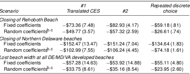
Point estimates and standard errors for the three welfare sce-narios (1997 dollars per respondent per season) are presented in Table 4. Columns 2 and 3 present the translated CES and sec-ond specication estimates, respectively. To evaluate whether our demand system models generate qualitatively different pol-icy inference from the discrete choice RUM-based strategies that dominate current empirical practice, column 4 presents welfare estimates from repeated discrete choice RUM models (e.g., Morey et. al. 1993) that are generated by the conditional welfare measurement procedure outlined in von Haefen (2003). The repeated discrete choice models assume (1) the recreation season can be decomposed into 75 separable choice occasions; (2) each individual on each choice occasion makes a discrete choice among the 62 beaches and an option not to recreate; (3) preferences for a beach (and the outside alternative) are a linear additive index of its price, attributes (a constant and de-mographic variables), and an i.i.d. Type I extreme value random draw; and (4) a subset of the parameters entering the indexes is statistically independent and normally distributed across the population. A table with parameter estimates for the specica-tions we consider in this paper is available from the authors upon request.
For each scenario xed and random parameter model esti-mates are presented together for comparison purposes. In all cases the estimates have plausible magnitudes and standard errors that suggest statistically signicant differences from 0. Additionally, a few general patterns emerge. Perhaps the most striking is that the inclusion of random coefcients decreases the magnitude of the estimated welfare effects for all mod-els and all scenarios. This is consistent with some empir-ical ndings in other random parameter applications (e.g., Petrin 2002; Phaneuf, Kling, and Herriges 1998) and sug-gests that the additional unobserved heterogeneity accounted for by random parameter models allows for a greater degree of substitutabilityamong goods and, as a result, smaller (absolute) economic values. Next, in spite of the statistical dominance of the second specication over the translated CES specica-tion, both demand system specications provide qualitatively
Table 4. Mean Seasonal Welfare Estimates (1997 dollars)a
#1 Repeated discrete
Scenario Translated CES #2 choice
Closing of Rehoboth Beach
Fixed coefcients ¡$73:36 (7:48) ¡$82:93 (4:17) ¡$59:18 (:81) Random coefcientsb;c ¡$49:77 (3:57) ¡$57:32 (2:59) ¡$26:61 (:74)
Closing of Northern Delaware beaches
Fixed coefcients ¡$152:47 (13:47) ¡$151:24 (7:04) ¡$134:64 (1:83) Random coefcientsb;c ¡$102:99 (7:55) ¡$106:24 (4:45) ¡$74:18 (1:61)
Lost beach width at all DE/MD/VA developed beaches
Fixed coefcients ¡$57:28 (14:63) ¡$53:92 (14:88) ¡$55:11 (4:80) Random coefcientsb;c ¡$33:75 (8:61) ¡$35:16 (8:54) ¡$23:95 (2:60)
a Robust standard errors based on 200 Krinsky and Robb (1986) simulations in parentheses. All estimates employ the sampling weights implied by the county-stratied sampling design.
b The xed coefcient Kuhn–Tucker welfare estimates were constructed with 25 simulations per observation. For the random coefcient Kuhn–Tucker welfare estimates, a total of 2;000 simulations were generated. The rst 1;000 simula-tions were discarded as burn-in and every 10th simulation thereafter was used to construct the estimates.
c The xed coefcient repeated discrete choice welfare estimates were constructed with 2;500 simulations per ob-servation. For the random coefcient discrete choice welfare estimates, a total of 13;500 simulations were generated. The rst 1;000 simulations were discarded as burn-in and every fth simulation thereafter was used to construct the estimates.
similar welfare measures for both the xed and the random parameter versions. Finally, our results suggest that the repeated discrete choice model generally produces welfare estimates that are smaller in absolute value. This result may in part reect the greater cross-site substitution patterns that can be character-ized within the discrete choice framework (particularly in the random parameter case) relative to our additively separable de-mand system model. However, this nding should be corrob-orated with results from other datasets and policy applications before general conclusions are drawn with condence.
7.2 Aggregate Welfare Estimates
The per person welfare measures can be used to construct aggregate estimates of the welfare impacts of the policies considered. The survey was designed to allow inference for the 576;246 Delaware residents 16 years and older in 1997. Because the mean estimates in Table 4 incorporate the sam-pling weights implied by the stratied random samsam-pling de-sign, multiplying the per person estimates by the population provides an estimate of the population welfare impact. These aggregate losses can be quite large for the scenarios considered. For example, our preferred demand system model (specica-tion 2 with random parameters) suggests an aggregate welfare loss of $33.1 million for Delaware residents for the closure of Rehoboth Beach for one season, and losses of $61.3 million for the closure of all northern beaches. The erosion losses are also substantial, estimated at $20.1 million per season for lost beach width.
Two caveats should be attached to these population welfare estimates. We have assumed that nonresponse to the survey in-strument was randomly assigned throughout the Delaware pop-ulation. If in fact beach visitors were more likely to respond to the survey than nonvisitors, the aggregate estimates are likely biased upward. In addition, these aggregate welfare measures do not reect the losses accruing to multiday and side trip users as well as nonresidentsof Delaware. For a full accounting of the total welfare impact of the proposed policies to all beach users, the welfare impacts to these other groups should be added to the estimates presented here.
8. CONCLUSION
Our general conclusion from the research presented in this article is that the demand system framework represents a viable strategy for modeling consumer choice and generating Hicksian welfare measures for individual or household level applications with many quality-differentiated goods. Using Monte Carlo estimation and welfare construction procedures, we present empirical results from a beach recreation application that demonstrate how this can be accomplished. Our methodolog-ical approach and empirmethodolog-ical ndings suggest that the demand system framework, which fully integrates the intensive and extensive margins of consumer choice within a behaviorally consistent framework, represents a genuine alternative to the RUM-based strategies that dominate current empirical practice. Numerous extensions to our approach are possible, and we discuss two in closing. Relaxing the assumption that pref-erences are additively separable represents a signicant area
for future work. From a computational perspective relaxing additive separability without jeopardizing the demand system framework’s tractability in estimation and welfare construction for applications with many goods represents a formidable task. However, our sense is that progress in this area is possible. In addition, our representation of the consumer’s problem as-sumes that all Delaware residents consider all 62 beaches in the Mid-Atlantic region. Introspection, however, suggests that it is doubtful that all individuals seriously consider all beaches. In the marketing literature discrete choice statistical models have been developed that build on Manski’s (1977) original formula-tion of the individual’s choice process and formally model the individual’s rst-stage formulation of his or her “consideration set” as well as his or her second-stage conditional choice (e.g., Ben-Akiva and Boccara 1995). Augmenting the demand system framework developed in this article with a model of the individ-ual’s consideration set formulation process would represent an innovation that may more accurately represent how individuals make choices.
ACKNOWLEDGMENTS
We thank Kerry Smith, Matt Massey, and seminar partici-pants at North Carolina State University, the University of Arizona, the University of California at Santa Barbara, the Environmental Protection Agency (EPA), the Second World Congress of Environmental and Resource Economists, the 57th European Meeting of the Econometric Society, the Heartland Environmental and Resource Economics Workshop, and the Stanford University Workshop on Equilibrium Modeling Ap-proaches at the Boundaries of Industrial Organization, Public Economics, and Environmental Economics for comments and suggestions. All remaining errors are our own. von Haefen ac-knowledges support from his former employer, the Bureau of Labor Statistics (BLS), Phaneuf acknowledges support from the EPA through contract #R826615010,and Parsons acknowl-edges support from the National Oceanic and Atmospheric Ad-ministration (NOAA) through a Delaware Sea Grant. The views expressed in this article are the authors alone and in no way rep-resent the views of the BLS, EPA, or NOAA.
[Received March 2002. Revised March 2003.]
REFERENCES
Ben-Akiva, M., and Boccara, B. (1995), “Discrete Choice Models With Latent Choice Sets,”International Journal of Research in Marketing, 12, 9–24. Berry, S., Levinsohn, J., and Pakes, A. (1995), “Automobile Prices in Market
Equilibrium,”Econometrica, 63, 841–890.
Bradford, D., and Hildebrandt, G. (1977), “Observable Preferences for Public Goods,”Journal of Public Economics, 8, 111–131.
Chiang, J., and Lee, L. F. (1992), “Discrete/Continuous Models of Consumer Demand With Binding Non-Negativity Constraints,”Journal of Economet-rics, 54, 79–93.
Chib, S., and Greenberg, E. (1995), “Understanding the Metropolis–Hastings Algorithm,”American Statistician, 49, 327–335.
Deacon, R., and Kolstad, C. (2000), “Valuing Beach Recreation Lost in Envi-ronmental Accidents,”Journal of Water Resources Planning and Manage-ment, 126, 374–381.
Feather, P., Hellerstein, D., and Tomasi, T. (1995), “A Discrete-Count Model of Recreation Demand,”Journal of Environmental Economics and Manage-ment, 29, 214–227.
Gelman, A., Carlin, J., Stern, H., and Rubin, D. (1995),Bayesian Data Analysis, London: Chapman & Hall.
Gourieroux, C., and Monfort, A. (1996),Simulation-Based Econometric Meth-ods, New York: Oxford University Press.
Griliches, Z. (1964), “Notes on the Measurement of Price and Quality Changes,” inModels of Income Determination, NBER Studies in Income and Wealth, Vol. 28, Princeton, NJ: Princeton University Press.
Hanemann, W. M. (1978), “A Theoretical and Empirical Study of the Recre-ation Benets From Improving Water Quality in the Boston Area,” Ph.D. dissertation, Harvard University.
(1984), “Discrete/Continuous Models of Consumer Demand,” Econo-metrica, 52, 541–561.
Hausman, J. A., Leonard, G. K., and McFadden, D. (1995), “A Utility-Consistent, Combined Discrete Choice and Count Data Model: Assessing Recreational Use Losses Due to Natural Resource Damage,”Journal of Pub-lic Economics, 56, 1–30.
Herriges, J. A., and Kling, C. L. (1999), “Nonlinear Income Effects in Random Utility Models,”Review of Economics and Statistics, 81, 62–72.
Krinsky, I., and Robb, A. (1986), “On Approximating the Statistical Properties of Elasticities,”Review of Economics and Statistics, 68, 715–719.
Lee, L. F., and Pitt, M. (1986), “Microeconomic Demand Systems With Bind-ing Non-Negativity Constraints: The Dual Approach,”Econometrica, 54, 1237–1242.
Mäler, K. G. (1974),Environmental Economics: A Theoretical Inquiry, Balti-more: Johns Hopkins University Press for Resources for the Future. Manski, C. (1977), “The Structure of Random Utility Models,”Theory and
Decision, 8, 229–254.
Massey, D. M. (2001), “Heterogeneous Preferences in Random Utility Models of Recreation Demand,” Ph.D. dissertation, University of Delaware. McFadden, D. (1974), “Conditional Logit Analysis of Qualitative Choice
Be-havior,” inFrontiers in Econometrics, ed. P. Zarembka, New York: Academic Press.
(2001), “Economic Choices,” American Economic Review, 91, 351–378.
Morey, E., Rowe, R., and Watson, M. (1993), “A Repeated Nested-Logit Model of Atlantic Salmon Fishing,”American Journal of Agricultural Economics, 75, 578–592.
Neary, J., and Roberts, K. (1980), “The Theory of Household Behavior Under Rationing,”European Economic Review, 13, 25–42.
Nevo, A. (2001), “Measuring Market Power in the Ready-to-Eat Cereal Indus-try,”Econometrica, 62, 307–342.
Parsons, G., Jakus, P., and Tomasi, T. (1999), “A Comparison of Welfare Esti-mates From Four Models for Linking Seasonal Recreation Trips to Multino-mial Logit Models of Choice,”Journal of Environmental Economics and Management, 38, 143–157.
Parsons, G., and Kealy, M. J. (1995), “A Demand Theory for Number of Trips in a Random Utility Model of Recreation,”Journal of Environmental Eco-nomics and Management, 29, 357–367.
Parsons, G., and Massey, D. M. (2003), “A Random Utility Model of Beach Recreation,” inThe New Economics of Outdoor Recreation, eds. N. Hanley, W. D. Shaw, and R. E. Wright. Northhampton, MA: Edward Elgar. Parsons, G., Massey, D. M., and Tomasi, T. (1999), “Familiar and Favorite Sites
in a Random Utility Model of Beach Recreation,” Marine Resource Eco-nomics, 14, 299–315.
Petrin, A. (2002), “Quantifying the Benets of New Products: The Case of the Mini-Vans,”Journal of Political Economy, 110, 705–729.
Phaneuf, D. J. (1999). “A Dual Approach to Modeling Corner Solutions in Recreation Demand,”Journal of Environmental Economics and Manage-ment, 37, 85–105.
Phaneuf, D. J., Kling, C. L., and Herriges, J. A. (1998), “Valuing Water Quality Improvements Using Revealed Preference Methods When Corner Solutions Are Present,”American Journal of Agricultural Economics, 80, 1025–1031. (2000), “Estimation and Welfare Calculations in a Generalized Cor-ner Solution Model With an Application to Recreation Demand,”Review of Economics and Statistics, 82, 83–92.
Phaneuf, D. J., and Smith, V. K. (2003), “Recreation Demand Models,” forth-coming in Handbook of Environmental Economics, eds. K. Mäler and J. Vincent.
Pollak, R., and Wales, T. (1991), “The Likelihood Dominance Criteria,”Journal of Econometrics, 47, 227–242.
(1992), Demand System Specication and Estimation, New York: Oxford University Press.
Small, K., and Rosen, H. (1981), “Applied Welfare Economics With Discrete Choice Models,”Econometrica, 49, 105–130.
Train, K. E. (2003),Discrete Choice Analysis With Simulation, Cambridge, U.K.: Cambridge University Press.
von Haefen, R. H. (2003), “Incorporating Observed Choice Into the Construc-tion of Welfare Measures From Random Utility Models,”Journal of Envi-ronmental Economics and Management, 45, 145–165.
Wales, T., and Woodland, A. (1983), “Estimation of Consumer Demand Sys-tems With Binding Non-Negativity Constraints,”Journal of Econometrics, 21, 263–285.