Manajemen | Fakultas Ekonomi Universitas Maritim Raja Ali Haji jbes%2E2009%2E07227

(1)

Full Terms & Conditions of access and use can be found at

http://www.tandfonline.com/action/journalInformation?journalCode=ubes20

Download by: [Universitas Maritim Raja Ali Haji] Date: 11 January 2016, At: 22:57

Journal of Business & Economic Statistics

ISSN: 0735-0015 (Print) 1537-2707 (Online) Journal homepage: http://www.tandfonline.com/loi/ubes20

Heteroscedastic Transformation Models With

Covariate Dependent Censoring

Shakeeb Khan, Youngki Shin & Elie Tamer

To cite this article: Shakeeb Khan, Youngki Shin & Elie Tamer (2011) Heteroscedastic

Transformation Models With Covariate Dependent Censoring, Journal of Business & Economic Statistics, 29:1, 40-48, DOI: 10.1198/jbes.2009.07227

To link to this article: http://dx.doi.org/10.1198/jbes.2009.07227

Published online: 01 Jan 2012.

Submit your article to this journal

Article views: 127

(2)

Heteroscedastic Transformation Models With

Covariate Dependent Censoring

Shakeeb KHAN

Department of Economics, Duke University, Durham, NC 27708-0097 (shakeebk@econ.duke.edu)

Youngki SHIN

Department of Economics, University of Western Ontario, London, ON N6A 5C2, Canada (yshin29@uwo.ca)

Elie TAMER

Department of Economics, Northwestern University, Evanston, IL 60208 (tamer@northwestern.edu)

In this article we propose an inferential procedure for transformation models with conditional het-eroscedasticity in the error terms. The proposed method is robust to covariate dependent censoring of arbitrary form. We provide sufficient conditions for point identification. We then propose an estimator and show that it is√n-consistent and asymptotically normal. We conduct a simulation study that reveals ade-quate finite sample performance. We also use the estimator in an empirical illustration of export duration, where we find advantages of the proposed method over existing ones.

KEY WORDS: Conditional heteroscedasticity; Rank estimation; Transformation model.

1. INTRODUCTION

The monotone transformation model is usually expressed as:

T(yi)=x′iβ0+εi, (1)

whereyi is a scalar dependent variable,xi is anl-dimensional vector of covariates, and εi is an unobservable error term whose distribution is unknown. The function T(_·)is unspeci-fied, but assumed to be monotone. The object of interest is the l-dimensional parameter vectorβ0. We assume that we have a

sample of iid observations.

In this article we consider the monotone transformation model with a general form of random censoring and condi-tional heteroscedasticity.We motivate this problem in the con-text of duration analysis. It can be shown that popular duration models, such as an accelerated failure time model, a propor-tional hazard model, and a mixed proporpropor-tional hazard model, are specific examples of the transformation model (seeRidder 1990). Thus, applying the transformation model will reduce the model specification error that might be caused by a specific haz-ard assumption. In duration data, however, censoring arises nat-urally because of a data collection procedure, and it may easily depend on covariates. For instance, a censoring variable of un-employment duration data may possibly depend on individual characteristics such as age, occupation, education, and so on. Also, conditional heteroscedasticity is quite common in such an economic dataset. Moreover, the presence of heteroscedas-ticity in nonlinear models can lead to inconsistency. Hence, the estimator proposed here fills a gap in the literature on censored models in that it is robust to both random censoring and het-eroscedasticity.

There is a large volume of the literature on estimating the transformation model, but no estimator allows for both a gen-eral form of random censoring and conditional heteroscedastic-ity simultaneously. The maximum rank correlation (MRC) esti-mator byHan(1987) and the monotone rank estimator (MRE) byCavanagh and Sherman(1998) can only be applied to special

forms of conditional heteroscedasticity, and do not allow for a censoring variable to be dependent on covariates in an arbitrary way.Khan(2001) proposed the quantile rank estimator (QRE) for a heteroscedastic transformation model, but it still does not allow for random censoring. Recently,Khan and Tamer(2007) proposed the partial rank estimator (PRE) that allows for ran-dom censoring, but it assumes that the error termεibe distrib-uted independently of the covariatesxi.

The two-stage partial rank estimation procedure can ac-commodate data with random censoring and conditional het-eroscedasticity. The new estimator shares the same advantages of usual rank estimators, so it does not require a specific er-ror distribution, and satisfies√n-consistency. In addition, it is consistent for random covariate dependent censoring and het-eroscedastic error terms under mild regularity conditions. The key condition is the median independence that is also adopted byManski(1985) for the maximum score estimator. The new estimator exploits the monotone property of a conditional me-dian function that is implied by the meme-dian independence. With-out any difficulty, it can be extended to any other quantile that is independent of covariates.

The rest of the article is organized as follows. In Section2, we introduce the model and estimation method. The asymptotic properties are also proposed in this section. The finite sample properties are investigated by means of Monte Carlo simula-tions in Section3. Section4 applies our estimator to export duration data and shows the advantages of our estimator over existing ones. Section5concludes and suggests future research areas. Technical proofs are presented in theAppendixunless it is helpful to understand the argument.

January 2011, Vol. 29, No. 1 DOI:10.1198/jbes.2009.07227

40

(3)

Khan, Shin, and Tamer: Heteroscedastic Transformation Models 41

2. ESTIMATION PROCEDURE AND

ASYMPTOTIC PROPERTIES

We modify Equation (1) slightly to allow for censoring. (We illustrate here identification for the one-sided censoring case. Similar arguments can be used to attain point identification re-sults for the double censoring case. SeeKhan and Tamer 2007.) The right-censored transformation model can be expressed as:

T(vi)=min(xi′β0+εi,ci), (2)

di=1(xi′β0+εi≤ci), (3)

where 1(_·)is an indicator function, ci is a random censoring variable that may depend onxi in an arbitrary way,di is a bi-nary random variable that indicates if the observation is cen-sored or not, andvi is a new dependent variable. The variable viisT−1(x′_iβ0+εi)for uncensored observations, which isyiin the original transformation model. For censored observations, viisT−1(ci).Observations are composed of(l+2)-dimensional vectors(vi,di,x′_i), and satisfy the iid assumption.

Random censoring models were studied widely in both econometrics and statistics, especially related to covariate de-pendent censoring (seeKhan and Tamer 2007and references therein). Although the PRE proposed by Khan and Tamer

(2007) is robust to covariate dependent censoring in the cen-sored transformation model, it requires that the error termεibe distributed independently of the covariatexi.This assumption may be overly restrictive in the sense that it rules out any form of conditional heteroscedasticity. In this article we relax the in-dependence assumption by assuming only a quantile ofǫi, say the median, is independent of the covariates. To permit random covariate dependent censoring, we now make the assumption that the random variablesciandǫiare statistically independent givenxi.

First, we establish an identification result and propose a median partial rank estimator (MPRE). Then, we show that it satisfies√n-consistency and asymptotic normality. The new es-timator exploits the monotone property of the conditional me-dian function. Based on monotone meme-dian functions, we can construct a rank estimator analogously toHan(1987) andKhan and Tamer(2007). The key condition for point identification of the MRC is

Pr(fij≥0|xi,xj)≥Pr(fji≥0|xi,xj) ⇔ xi′β0≥xj′β0,

(4) for some functionsfijandfji. To motivate the new estimator, we first define the random variables:

y1i=di·vi+(1−di)·(+∞), (5)

y0i=vi, (6)

where we define 0×(_+∞)_≡0.Then, we can derive a part of Equation (4) by letting

fij=med(T(y1i)|xi)−med(T(y0j)|xj), (7)

and showing that

x_i′β0≥x′jβ0 ⇒ Pr(fij≥0|xi,xj)=1. (8)

To show this, let m1(xi) and m0(xj) denote conditional me-dian functions of T(y1i) and T(y0j) given xi and xj, respec-tively. Then, we can rewrite the conditional probability Pr(fij≥ 0|xi,xj)as:

Pr(fij≥0|xi,xj)=Pr(m1(xi)≥m0(xj)). (9)

Finally, Equation (8) holds from the following inequality that is true for allxi:

m0(xi)≤x′iβ0≤m1(xi). (10)

We next summarize the related regularity conditions and pro-pose the detailed identification result in Theorem2.1.

I1. LetSXdenote the support ofxi, and letX denote the set

X_{= {}x_∈SX: Pr(xi′β0≤ci|xi=x)=1}. (11)

Then,X _{has positive measure.}

I2. The random variable εi is distributed independently of the random variableciconditional onxi,and satisfies the median independence:

med(εi|xi)=0. (12)

I3. The support ofxiis not contained in a proper linear sub-space of Rl and the lth component of xi has an every-where positive Lebesgue density conditional on the re-maining components.

Condition I1 requires that there exists somexwith positive measure, such that the index valuexβ0is less than the

censor-ing variable for all support ofci. The condition can be seen as an extension of the assumption R.1 inPowell(1984) to a ran-dom censoring case. This condition always holds if the censor-ing variable is truncated and condition I3 is true. Condition I2 requires the conditional independence between the error term and the censoring variable. Also it assumes that the median of the error term is distributed independently of the covariatexi. Since this condition permits any relationship betweenεiandxi for other quantiles, conditional heteroscedasticity is allowed in the model. Condition I3 is the standard regularity condition for point identification in semiparametric literature. This condition is also adopted by the MRC and the maximum score estimator. Point identification is characterized by the following theo-rem, the proof for which is found in theAppendix:

Theorem 2.1. Suppose that the assumptions I1–I3 hold. LetyidenoteT−1(x′_iβ0+εi).Then we have

m0(xi)=m1(xi)=med(T(yi)|xi)=x′iβ0, (13)

if and only ifxi∈X.

The above result, along with the invariance of medians, sug-gests an (infeasible) rank estimator based on the conditional medians ofy0iandy1i. Thus, we will estimateβ0by

maximiz-The functionQn(β)exploitsKendall(1938)’s measure for rank correlation between median functions and indexes.

To construct a feasible estimation procedure, we replace the unknown median functions in the above estimator with

(4)

their nonparametric estimators. For these first stage estima-tors, we adopt the local polynomial approach introduced in

Chaudhuri (1991). For a detailed description of the estima-tor, see Chaudhuri (1991). Here, we simply let mˆδn,p

0 (xi)and

ˆ mδn,p

1 (xi)denote the local polynomial estimators where the

su-perscripts denote the bandwidth sequence (δn) and order of polynomial (p) used. Conditions onδnandpare stated in Theo-rem2.2characterizing the limiting distribution of our estimator ofβ0. To avoid the technical difficulty of dealing with a

smooth-ing parameter inside an indicator function, we define our het-eroscedasticity robust estimator of β0, denoted here asβˆht, as follows:

imating function to an indicator function (i.e., a cumulative distribution function), and hn denotes a sequence of positive constants, converging to 0 such that in the limit we have an indicator function. Finally, τ (_·)is a function that trims away values of the regressors where the median functions cannot be estimated precisely. For notational convenience, their presence will be suppressed hereafter and we explain conditions for them in theAppendix. This smoothing technique was introduced in the seminal work ofHorowitz(1992).

We next state the limiting distribution theory forβˆht. Our lim-iting distribution theory for this estimator is based on the set of assumptions that are similar to those imposed in Sherman

(1993) and Khan(2001). Specifically, the assumptions in the proof impose conditions on the bandwidth sequences and or-ders of smoothness of conditional median functions to ensure that our first step estimators of these functions converge uni-formly at a rate faster thann−1/4. Further assumptions imposed are analogous to those in Sherman (1993) to ensure the lim-iting objective function is sufficiently smooth (i.e., twice con-tinuously differentiable) inβso we can work with its quadratic approximation. We relegate these assumptions to theAppendix. The following theorem establishes that these additional as-sumptions, along with a stronger smoothness condition on the median function and further restrictions on the bandwidth se-quence, are sufficient for root-n consistency and asymptotic normality of the proposed estimator:

Theorem 2.2. Letxbe decomposed into continuous and dis-crete elements as(x(d),x(c))whose dimensions areldandlc, re-spectively. Assume thatp>3lc/2, and that in the first stage,k is set to int(p)and the bandwidth sequences satisfy√nδpn→0,

Then, under Assumptions A, B, Q, T, E, and SI listed in the

Appendix

The variance matrix can be consistently estimated by a nu-merical derivative form (see Sherman 1993 and Khan and Tamer 2007) or a kernel method. One may also estimate it from the bootstrap that we adopt in Section4. In fact, we find that terms involving numerical derivatives are quite sensitive to the choice of the smoothing parameter. Thus, we recommend the bootstrap to escape from an arbitrary conclusion depending on a smoothing parameter.

3. MONTE CARLO SIMULATION

In this section we investigate small sample properties of the proposed estimator by conducting a simple Monte Carlo sim-ulation study. The base design is a censored transformation model with two covariates

T(vi)=min(x1i+x2iβ0+εi,ci),

di=1(x1i+x2iβ0+εi≤ci),

wherex1i andx2i are distributed as standard normal, and chi-squared with 1 degree of freedom. The coefficient ofx1iis nor-malized as 1 andβ0is set to be 0.5. The transformation

func-tionT(_·)is either the identity or the log function. For the error distribution, we consider the normal distribution and the Stu-dent’st distribution. Finally, we consider both covariate inde-pendent and covariate deinde-pendent censored models. Therefore, there are the following eight simulation designs in total:

Design 1. T(v)₌v, εi∼0.5×N(0,1), andci∼lognormal.

All designs with odd numbers have homoscedastic error terms and covariate independent censoring variables. In the remain-ing designs with even numbers, we have both conditional het-eroscedastic errors and covariate dependent censoring.

Tables1through4 summarize the simulation results. Each table contains two designs in order. We conducted 401 repli-cations for a simulation design with sample sizes of 50, 100, 200, and 400. In the first stage of MPRE, we estimate condi-tional median functions by applying the nonparametric method inChaudhuri(1991). We fit the model as a constant function and use the optimal bandwidth c1n−6.5 for a constant c1. In

the second stage, we estimateβ0by maximizing the objective

function of the MPRE in Equation (15). The cumulative den-sity function of the standard normal distribution is used for the kernel function. For the bandwidth of the kernel function, we again use the optimal bandwidthc2(n(n−1))−1/5.

Con-stantsc1 andc2are chosen by the rule of thumb explained in

Fan and Gijbels(1996). A grid search method is applied for an

(5)

Table 1. Simulations results: linear models with Normal distribution

Mean bias Median bias RMSE MAD

Covariate independent

50 obs. MPRE 0.0106 −0.0100 0.1573 0.1224

PRE 0.0493 0.0000 0.2706 0.1955

MRC 0.0281 ₋0.0100 0.2159 0.1609

100 obs. MPRE ₋0.0025 ₋0.0100 0.1142 0.0895

PRE 0.0146 0.0100 0.1560 0.1217

MRC 0.0107 0.0100 0.1361 0.1033

200 obs. MPRE −0.0194 −0.0200 0.0781 0.0626

PRE −0.0016 0.0000 0.0970 0.0755

MRC −0.0026 0.0000 0.0831 0.0659

400 obs. MPRE −0.0062 −0.0100 0.0536 0.0431

PRE 0.0052 0.0000 0.0639 0.0499

MRC 0.0051 0.0100 0.0528 0.0422

Covariate dependent

50 obs. MPRE −0.0611 −0.0500 0.1458 0.1074

PRE 0.1206 0.1000 0.1782 0.1343

MRC 0.1115 0.1000 0.1514 0.1193

100 obs. MPRE ₋0.0495 ₋0.0400 0.0899 0.0703

PRE 0.1045 0.1000 0.1261 0.1071

MRC 0.1068 0.1000 0.1236 0.1076

200 obs. MPRE ₋0.0255 ₋0.0200 0.0548 0.0419

PRE 0.1071 0.1000 0.1176 0.1072

MRC 0.1077 0.1100 0.1162 0.1077

400 obs. MPRE −0.0183 −0.0200 0.0336 0.0264

PRE 0.1003 0.1000 0.1060 0.1003

MRC 0.0999 0.1000 0.1043 0.0999

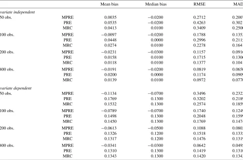
Table 2. Simulations results: linear models with Student-tdistribution

50 obs. MPRE 0.0035 −0.0200 0.2712 0.2007

PRE 0.0535 ₋0.0200 0.4263 0.3021

MRC 0.0413 0.0100 0.3409 0.2500

100 obs. MPRE −0.0097 −0.0200 0.1788 0.1353

PRE 0.0448 0.0000 0.2996 0.2115

MRC 0.0274 0.0100 0.2278 0.1641

200 obs. MPRE ₋0.0231 ₋0.0300 0.1157 0.0916

PRE 0.0158 0.0100 0.1715 0.1306

MRC 0.0118 0.0100 0.1377 0.1041

400 obs. MPRE −0.0191 −0.0200 0.0819 0.0650

PRE 0.0200 0.0000 0.1174 0.0909

MRC 0.0139 0.0100 0.0972 0.0770

50 obs. MPRE −0.1134 −0.0700 0.3496 0.2322

PRE 0.1769 0.1300 0.3202 0.2189

MRC 0.1532 0.1300 0.2574 0.1859

100 obs. MPRE −0.0789 −0.0700 0.1740 0.1249

PRE 0.1498 0.1300 0.2048 0.1599

MRC 0.1450 0.1300 0.1769 0.1474

200 obs. MPRE ₋0.0613 ₋0.0500 0.1088 0.0803

PRE 0.1326 0.1200 0.1518 0.1335

MRC 0.1317 0.1200 0.1476 0.1319

400 obs. MPRE ₋0.0341 ₋0.0300 0.0642 0.0495

PRE 0.1310 0.1300 0.1419 0.1310

MRC 0.1343 0.1300 0.1420 0.1343

(6)

Table 3. Simulations results: log-linear models with Normal distribution

50 obs. MPRE 0.0075 0.0000 0.1532 0.1198

PRE 0.0462 0.0000 0.2781 0.1976

MRC 0.0188 0.0000 0.2263 0.1646

100 obs. MPRE 0.0003 −0.0100 0.1084 0.0845

PRE 0.0168 0.0100 0.1471 0.1109

MRC 0.0097 0.0100 0.1234 0.0936

200 obs. MPRE −0.0046 −0.0100 0.0733 0.0574

PRE 0.0002 ₋0.0100 0.1047 0.0816

MRC −0.0003 0.0000 0.0825 0.0643

400 obs. MPRE −0.0020 0.0000 0.0559 0.0439

PRE 0.0045 0.0000 0.0675 0.0528

MRC 0.0041 0.0000 0.0543 0.0428

50 obs. MPRE ₋0.0377 ₋0.0400 0.1319 0.0998

PRE 0.1060 0.1000 0.1554 0.1232

MRC 0.1119 0.1000 0.1499 0.1215

100 obs. MPRE ₋0.0390 ₋0.0400 0.0887 0.0692

PRE 0.1112 0.1000 0.1349 0.1133

MRC 0.1097 0.1100 0.1287 0.1108

200 obs. MPRE −0.0191 −0.0200 0.0495 0.0381

PRE 0.1027 0.1000 0.1144 0.1031

MRC 0.1009 0.1000 0.1092 0.1009

400 obs. MPRE −0.0125 −0.0100 0.0327 0.0251

PRE 0.1028 0.1000 0.1081 0.1028

MRC 0.1006 0.1000 0.1051 0.1006

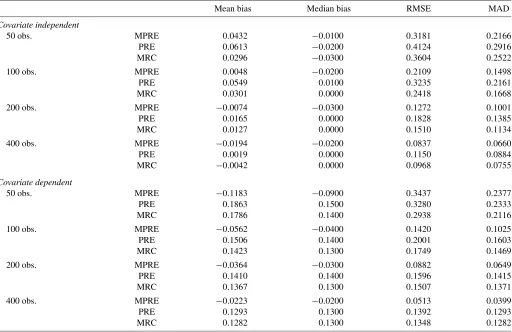
Table 4. Simulations results: log-linear models with Student-tdistribution

50 obs. MPRE 0.0432 −0.0100 0.3181 0.2166

PRE 0.0613 ₋0.0200 0.4124 0.2916

MRC 0.0296 −0.0300 0.3604 0.2522

100 obs. MPRE 0.0048 −0.0200 0.2109 0.1498

PRE 0.0549 0.0100 0.3235 0.2161

MRC 0.0301 0.0000 0.2418 0.1668

200 obs. MPRE ₋0.0074 ₋0.0300 0.1272 0.1001

PRE 0.0165 0.0000 0.1828 0.1385

MRC 0.0127 0.0000 0.1510 0.1134

400 obs. MPRE −0.0194 −0.0200 0.0837 0.0660

PRE 0.0019 0.0000 0.1150 0.0884

MRC −0.0042 0.0000 0.0968 0.0755

50 obs. MPRE −0.1183 −0.0900 0.3437 0.2377

PRE 0.1863 0.1500 0.3280 0.2333

MRC 0.1786 0.1400 0.2938 0.2116

100 obs. MPRE −0.0562 −0.0400 0.1420 0.1025

PRE 0.1506 0.1400 0.2001 0.1603

MRC 0.1423 0.1300 0.1749 0.1469

200 obs. MPRE ₋0.0364 ₋0.0300 0.0882 0.0649

PRE 0.1410 0.1400 0.1596 0.1415

MRC 0.1367 0.1300 0.1507 0.1371

400 obs. MPRE ₋0.0223 ₋0.0200 0.0513 0.0399

PRE 0.1293 0.1300 0.1392 0.1293

MRC 0.1282 0.1300 0.1348 0.1282

(7)

optimization algorithm. We evaluate the objective function on 401 equispaced points on the interval_[−2,2_].For comparison, the performance of the PRE and the MRC estimator is also ex-amined. Again, the grid search method is used for finding the maximum of the sample objective function.

Overall, the MPRE estimator shows good finite sample per-formance in all simulation experiments. First, the lower panels of each table show that the MPRE only satisfies the paramet-ric convergence rate as expected from the theory. The biases of the PRE and the MRC do not seem to decrease much, and their root mean square errors (RMSE’s) decrease slowly either when the sample size increases from 200 or to 400. Considering dif-ferent transformation functions and error distributions used in the simulations, this result reveals the advantage of the MPRE. Furthermore, the MPRE also shows better performance in co-variate independent designs. In the upper panels, the MPRE has the lowest RMSE’s besides the 400 observations with normal errors. Especially, it outperforms the other two estimators when observations are as small as 50 or 100.

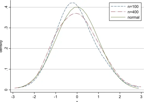
In this simulation study, we also check the accuracy of the normal approximation in finite samples. We standardize the simulated estimates using the sample mean and variance, and compare its percentiles, skewness, and kurtosis with those of the standard normal distribution in each simulation design. Overall, the normal approximation appears to be appropriate when the sample size is over 200. For the sample sizes of 50 and 100, however, we find some cases of large skewness (De-sign 7) and/or heavy tails (De(De-signs 4 and 7). For better interpre-tation, we also estimate their probability density functions (pdf) using the nonparametric kernel method. Figure1shows the es-timation results of Design 7 with 100 and 400 observations. (The tables and graphs for other Designs are available upon re-quest from the authors.) Again, we confirm that the sampling distribution is approximately normal in all cases. However, if a researcher has relatively small observations in data, or wants more robust results, we recommend using the bootstrap for the inference.

Consequently, the results from our simulation study indicate that the MPRE introduced in this article performs well for het-eroscedastic transformation models with covariate dependent random censoring. Thus, it can be applied to empirical settings with flexible restrictions as we will see in the next section.

Figure 1. Accuracy of Normal approximation: Design 7. The online version of this figure is in color.

4. EMPIRICAL ILLUSTRATION: EXPORT DURATION

To help illustrate the proposed method, we consider a simple model of export duration with Chilean plant-level data. Specif-ically, we estimate the effects of plant size,capital size, and import statuson export duration. From the original panel data from 1989 to 1997, we collected 1868 observations of plants that had exported at least once during this period. Observa-tions were recorded as censored duration if the plant exited the market while exporting some goods or kept the export status in 1997. The plant size was measured by the logarithm of the number of employees, and the capital size by the logarithm of the real capital. All covariates are from the values in the year when they started exporting. Table 5summarizes the descrip-tive statistics of the dataset.

In the data, we can expect that censoring will depend on co-variates. As an initial check of this point, we ran a simple linear regression of duration on other covariates using the subsam-ple of censored observations. We find that export duration of the censored subsample depends on plant size and import sta-tus very significantly (their t-statistics are 9.86 and 4.37, re-spectively). In addition, the data show the high censoring ratio of 72%, which helps reveal the bias, if any, from the covari-ate dependency. By the White test both on the level of duration and on the logarithm of it, we also checked the heteroscedas-ticity, which is the rule rather than the exception in the eco-nomic dataset. As expected, we can easily reject the null of homoscedasticity with thep-value less than 1% in both cases. Therefore, we can think of three different causes of bias: (1) co-variate dependent censoring, (2) heteroscedastic error terms, and (3) misspecification of the transformation function and the error distribution.

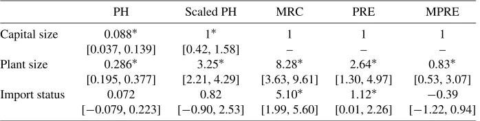
To reveal these different biases, we estimate the model using four different estimation methods: Cox’s proportional hazard (PH), MRC, PRE, and MPRE. The PH model was estimated by the standard maximum likelihood method, and we changed its scale to compare them with the results of the remaining rank estimators. The simulated annealing method was adopted for point estimates of rank estimators and 90% confidence inter-vals, denoted in square brackets, were constructed by the boot-strap method.

We summarize the estimation result in Table 6. There are three points to be noted. First, we observe heteroscedasticity bias from comparing the estimation results of the PRE and the MPRE. The effect of plant size in the PRE is three times larger than that in the MPRE. Furthermore, import status has a signif-icant positive effect in the PRE, which is not true in the MPRE. Second, the difference between the MRC and the PRE can be

Table 5. Descriptive statistics

Variable Mean Std. dev. Min Max

Export duration 3.49 2.36 1 7 Completed duration

(0 if censored) 0.28 0.45 0 1 Capital size: log(real capital) 11.97 1.85 4.82 19 Plant size: log(# of employees) 4.43 1.04 2.30 8.27 Import status (0 if no import) 0.46 0.50 0 1

Number of observations: 1868

(8)

Table 6. Estimation results of unemployement duration data

PH Scaled PH MRC PRE MPRE

Capital size 0.088∗ 1∗ 1 1 1

[0.037, 0.139] [0.42, 1.58] – – – Plant size 0.286∗ 3.25∗ 8.28∗ 2.64∗ 0.83∗

[0.195, 0.377] [2.21, 4.29] [3.63, 9.61] [1.30, 4.97] [0.53, 3.07] Import status 0.072 0.82 5.10∗ 1.12∗ −0.39

[₋0.079, 0.223] [₋0.90, 2.53] [1.99, 5.60] [0.01, 2.26] [₋1.22, 0.94]

NOTE: The 90% confidence intervals denoted in square brackets were constructed by the bootstrap method. The asterisk mark * denotes that the estimate is significant at 10% level.

seen as the bias from the covariate dependent censoring. The MRC estimation reports three to four times larger effects of the covariates than the PRE. Third, the different result of the scaled PH adds a model misspecification bias into the previous biases. This result implies that the error term may not follow the Type I extreme value distribution, which is an underlying assumption of Cox’s PH model.

This empirical illustration shows that the MPRE has an ad-vantage over existing methods when censored duration depends on covariates and the censoring ratio is high. Therefore, consid-ering that heteroscedastic errors are common in economic data, we recommend estimating a censored duration model by the MPRE for robust results.

5. CONCLUSION

In this article we consider a censored transformation model with conditional heteroscedasticity. To estimate the model, we propose the median partial rank estimation procedure. It is shown that the proposed estimator satisfies√n-consistency and asymptotic normality. We also investigate its finite sample prop-erties through a Monte Carlo simulation study and show that it works appropriately in small samples. For empirical illustra-tion, we estimate a model of export duraillustra-tion, which shows that the MPRE performs better than existing methods.

We conclude this article by suggesting areas of future re-search. First, it will be useful to formally construct an estima-tor for the transformation functionT(_·).It can be achieved by modifying the rank estimation procedure inChen(2002). Sec-ond, one may think of an extended model with functional co-efficients, i.e., linear coefficients are nonparametric functions of additional covariates. These nonparametric functional coef-ficients can be estimated by adopting some localizing meth-ods.

APPENDIX

A.1 Assumptions for the Asymptotic Normality

Assumptions on the Regressors.

B1. The sequence of(l₊2)-dimensional vectors(vi,di,xi) are independent and identically distributed.

B2. The regressor vectorxihas support that is a subset ofRl. We order the components ofxi so it can be written as xi=(xi(d),xi(c))′. Letlcdenote dim(xi(c)). Assume that 1≤lc≤land that the supportxi(c)is a convex subset of

Rlc _{and has nonempty interior. Assume that the support}

ofxi(d)is a finite number of points lying inRl−lc. We let fX(x)denote the product of the conditional (Lebesgue) density ofx(_ic)givenx(_id)[denoted byf_X(c)_|_X(d)₌_x(d)(x(c))]

and the marginal probability mass function ofX(d) [de-noted byf_X(d)(x(d))].

B3. f_X(c)_|_X(d)(x(c))is continuous and bounded on the support

ofx(_ic).

B4. Assume thatX_t₌X_t₍_l₋₁₎_×X_tl_{, where}X_t₍_l₋₁₎ _andX_tl

are compact subsets with nonempty interiors of the sup-ports of the firstl₋1 components, and thelth compo-nent ofxi, respectively. For eachx∈Xt, denote its first l₋1 components byx(l−1).Xt is assumed to have the following properties:

B4.1. X_t_{is not contained in any proper linear subspace}

ofRl.

B4.2. fX(x)≥ǫ0>0∀x∈Xt, for some constantǫ0.

Assumptions on the Median Functions.

Q1. For any valuex(d) _{in the support of} _x(d)

i ,mj(·)for j= 0,1 isktimes differentiable inx(_ic). Letting∇kmj(x(c), x(d))denote the vector ofkth order derivatives ofmj(·) inx(_ic), we assume the following Lipschitz condition:

∇kmjx₁(c),x(d)−∇kmjx(₂c),x(d)≤K

x(₁c)₋x(₂c) γ

,

for all values x(₁c),x₂(c) in the support of x_i(c), where · denotes the Euclidean norm, γ_∈(0,1_], and K_is

some positive constant. In the theorems to follow, we let p₌k₊γdenote theorder of smoothnessof the median function.

Assumptions on the Trimming Function.

T. The trimming functionτ:Rl→R+is continuous, bound-ed, and bounded away from 0 on its support, denoted byX_τ_{, a compact subset of}_Rl_.

Assumptions on the Median Residual Terms.

D1. Letu1i=y1i−m1(xi); in a neighborhood of 0,u1ihas a conditional (Lebesgue) density, denoted byfu1|Xi=x(·),

which is continuous and bounded away from 0 and in-finity for all values ofx_∈X_t_{. As a function of}_x,fu_|Xi=x

is Lipschitz continuous for all values ofu1i in a neigh-borhood of 0. Defineu0ianalogously and assume it has analogous properties.

(9)

Furthermore, we require conditions on the smoothness of the median functions. Letθdenote the subset of regression coeffi-cients reflecting the scale normalization and define

τq1(x, θ )=

Then we impose the following additional assumptions:

E1. For eachxin the support ofxi,τq1(x,·)is differentiable

of order 2, with Lipschitz continuous second derivative onN_.

E2. E_[∇2τq1(·, θ0)]is negative definite.

E3. For eachxin the support ofxi,τq2(x,·)is continuously

differentiable onN_.

E4. E_[∇1τq2(·, θ0)2]<∞.

Next, we impose conditions on the second stage smoothed indicator function and bandwidth:

SI1. The functionK(_·)is positive, strictly increasing, twice differentiable with bounded first and second derivatives, and satisfies the following:

First we show the necessity part. Suppose thatxi∈X.Then, we have

where the third equality follows from the hypothesis thatxi∈

X_{, i.e., Pr}(ci−x′iβ0≥0|xi)=1.Now we turn our attention to

where the third equality again follows from the hypothesis. Therefore, we can conclude that

A.3 Proof of Theorem2.2

The asymptotic properties follow from arguments that are very similar to those used inKhan(2001), so we only provide a sketch of the steps involved. First, we expand the kernel func-tion of the estimated median funcfunc-tions around the kernel of the true median functions in Equation (15), yielding the sum of the three components:

(10)

where we adopt the shorthand notation mˆ1i;m1i denotes ˆ

mδn,p

1 (xi),m1(xi), respectively, and∗denotes intermediate

val-ues.

First we deal with Equation (A.3). It follows by uniform rates of convergence for median function estimators over com-pact sets (see, e.g.,Chaudhuri 1991), where these rates depend onp, δn, Assumptions SI1, SI2, and the rates imposed onδn,hn stated in the theorem.Rn(β)isop(1/n)uniformly overβwithin anOp(1/√n)neighborhood ofβ0.

Turning our attention to Hn(β), with the properties ofK(·) in Assumption SI1, we apply the arguments in lemma A.4 in

Khan(2001) that uniformly overβwithinop(1)neighborhoods ofβ0, we have

Hn(β)=(β−β0)′

1 n

n

i₌1

δ(y1i,y0i,xi)+op(1/n). (A.4)

Finally, with regard to Ŵn(β), we have, by the properties of K(_·),hn in Assumptions SI1, SI2, using identical argu-ments as in lemma A.3 inKhan(2001), that uniformly overβ withinop(1)neighborhoods ofβ0, we have

Ŵn(β)=1₂(β−β0)′Vq(β−β0)+op(1/n). (A.5)

Combining these three results, the limiting distribution of the estimator follows by applying lemma A.2 inKhan(2001).

ACKNOWLEDGMENTS

The authors thank the helpful comments provided by the co-editor, Serena Ng, and two anonymous referees. Hiro Kasahara

graciously provided the data used in the article. Any errors that remain are solely our responsibility.

[Received September 2007. Revised June 2009.]

REFERENCES

Cavanagh, C., and Sherman, R. (1998), “Rank Estimation for Monotonic Index Models,”Journal of Econometrics, 84 (2), 351–381. [40]

Chaudhuri, P. (1991), “Nonparametric Estimates of Regression Quantiles and Their Local Bahadur Representation,”The Annals of Statistics, 19, 760– 777. [42,48]

Chen, S. (2002), “Rank Estimation of Transformation Models,”Econometrica, 70 (4), 1683–1697. [46]

Fan, J., and Gijbels, I. (1996),Local Polynomial Modelling and Its Applica-tions, New York: Chapman & Hall. [42]

Han, A. (1987), “Non-Parametric Analysis of a Generalized Regression Model,”Journal of Econometrics, 35 (2), 303–316. [40,41]

Horowitz, J. L. (1992), “A Smoothed Maximum Score Estimator for the Binary Response Model,”Econometrica, 60, 505–531. [42]

Kendall, M. G. (1938), “A New Measure of Rank Correlation,”Biometrika, 30, 81–93. [41]

Khan, S. (2001), “Two-Stage Rank Estimation of Quantile Index Models,” Journal of Econometrics, 100, 319–355. [40,42,47,48]

Khan, S., and Tamer, E. (2007), “Partial Rank Estimation of Transformation Models With General Forms of Censoring,”Journal of Econometrics, 136 (1), 251–280. [40-42]

Manski, C. (1985), “Semiparametric Analysis of Discrete Response: Asymp-totic Properties of Maximum Score Estimation,”Journal of Econometrics, 27 (3), 313–334. [40]

Powell, J. L. (1984), “Least Absolute Deviations Estimation for the Censored Regression Model,”Journal of Econometrics, 25, 303–325. [41]

Ridder, G. (1990), “The Non-Parametric Identification of Generalized Accel-erated Failure-Time Models,”Review of Economic Studies, 57, 167–182. [40]

Sherman, R. (1993), “The Limiting Distribution of the Maximum Rank Corre-lation Estimator,”Econometrica, 61 (1), 123–137. [42]