Full Terms & Conditions of access and use can be found at
http://www.tandfonline.com/action/journalInformation?journalCode=ubes20
Download by: [Universitas Maritim Raja Ali Haji] Date: 12 January 2016, At: 23:27
Journal of Business & Economic Statistics
ISSN: 0735-0015 (Print) 1537-2707 (Online) Journal homepage: http://www.tandfonline.com/loi/ubes20
Realized Variance and Market Microstructure
Noise
Peter R Hansen & Asger Lunde
To cite this article: Peter R Hansen & Asger Lunde (2006) Realized Variance and Market
Microstructure Noise, Journal of Business & Economic Statistics, 24:2, 127-161, DOI: 10.1198/073500106000000071
To link to this article: http://dx.doi.org/10.1198/073500106000000071
Published online: 01 Jan 2012.
Submit your article to this journal
Article views: 690
View related articles
Meetings, Minneapolis, Minnesota, August 7–11, 2005.
Realized Variance and Market
Microstructure Noise
Peter R. H
ANSENDepartment of Economics, Stanford University, 579 Serra Mall, Stanford, CA 94305-6072 (peter.hansen@stanford.edu)
Asger L
UNDEDepartment of Marketing and Statistics, Aarhus School of Business, Fuglesangs Alle 4, 8210 Aarhus V, Denmark
We study market microstructure noise in high-frequency data and analyze its implications for the real-ized variance (RV) under a general specification for the noise. We show that kernel-based estimators can unearth important characteristics of market microstructure noise and that a simple kernel-based estimator dominates the RV for the estimation of integrated variance (IV). An empirical analysis of the Dow Jones Industrial Average stocks reveals that market microstructure noise is time-dependent and correlated with increments in the efficient price. This has important implications for volatility estimation based on high-frequency data. Finally, we apply cointegration techniques to decompose transaction prices and bid–ask quotes into an estimate of the efficient price and noise. This framework enables us to study the dynamic effects on transaction prices and quotes caused by changes in the efficient price.
KEY WORDS: Bias correction; High-frequency data; Integrated variance; Market microstructure noise; Realized variance; Realized volatility; Sampling schemes.
The great tragedy of Science—the slaying of a beautiful hypothesis by an ugly fact (Thomas H. Huxley, 1825–1895).
1. INTRODUCTION
The presence of market microstructure noise in high-frequen-cy financial data complicates the estimation of financial volatil-ity and makes standard estimators, such as the realized variance(RV), unreliable. Thus, from the perspective of volatil-ity estimation, market microstructure noise is an “ugly fact” that challenges the validity of theoretical results that rely on the ab-sence of noise. Volatility estimation in the preab-sence of market microstructure noise is currently a very active area of research. Interestingly, this literature was initiated by an article by Zhou (1996) that was published in this journal a decade ago and was in many ways 10 years ahead of its time.
The best remedy for market microstructure noise depends on the properties of the noise, and the main purpose of this arti-cle is to unearth the empirical properties of market microstruc-ture noise. We use a number of kernel-based estimators that are well suited for this problem, and our empirical analysis of high-frequency stock returns reveals the following ugly facts about market microstructure noise:
1. The noise is correlated with the efficient price. 2. The noise is time-dependent.
3. The noise is quite small in the Dow Jones Industrial Av-erage (DJIA) stocks.
4. The properties of the noise have changed substantially over time.
These four empirical “facts” are related to one another and have important implications for volatility estimation. The time dependence in the noise and the correlation between noise and efficient price arise naturally in some models on market
mi-crostructure effects, including (a generalized version of ) the bid–ask model by Roll (1984) (see Hasbrouck 2004 for a dis-cussion) and models where agents have asymmetric informa-tion, such as those by Glosten and Milgrom (1985) and Easley and O’Hara (1987, 1992). Market microstructure noise has many sources, including the discreteness of the data (see Harris 1990, 1991) and properties of the trading mechanism (see, e.g., Black 1976; Amihud and Mendelson 1987). (For additional ref-erences to this literature, see, e.g., O’Hara 1995; Hasbrouck 2004.)
The main contributions of this article are as follows: First, we characterize how the RV is affected by market microstruc-ture noise under a general specification for the noise that allows for various forms of stochastic dependencies. Second, we show that market microstructure noise is time-dependent and corre-lated with efficient returns. Third, we consider some existing theoretical results based on assumptions about the noise that are too simplistic, and discuss when such results provide reason-able approximations. For example, our empirical analysis of the 30 DJIA stocks shows that the noise may be ignored when in-traday returns are sampled at relatively low frequencies, such as 20-minute sampling. Assuming the noise is of an independent type seems to be reasonable when intraday returns are sampled every 15 ticks or so. Fourth, we apply cointegration methods to decompose transaction prices and bid/ask quotations into es-timates of the efficient price and market microstructure noise. The correlations between these estimated series are consistent with the volatility signature plots. The cointegration analysis enables us to study how a change in the efficient price dynami-cally affects bid, ask, and transaction prices.
© 2006 American Statistical Association Journal of Business & Economic Statistics April 2006, Vol. 24, No. 2 DOI 10.1198/073500106000000071
127
The interest for empirical quantities based on high-frequency data has surged in recent years (see Barndorff-Nielsen and Shephard 2007 for a recent survey). The RV is a well-known quantity that goes back to Merton (1980). Other empirical quantities include bipower variation and multipower varia-tion, which are particularly useful for detecting jumps (see Barndorff-Nielsen and Shephard 2003, 2004, 2006a,b; Ander-sen, Bollerslev, and Diebold 2003; Bollerslev, Kretschmer, Pig-orsch, and Tauchen 2005; Huang and Tauchen 2005; Tauchen and Zhou 2004), and intraday range-based estimators (see Christensen and Podolskij 2005). High-frequency–based quan-tities have proven useful for a number of problems. For ex-ample, several authors have applied filtering and smoothing techniques to time series of the RV to obtain time series for daily volatility (see, e.g., Maheu and McCurdy 2002; Barndorff-Nielsen, Nielsen, Shephard, and Ysusi 1996; Engle and Sun 2005; Frijns and Lehnert 2004; Koopman, Jungbacker, and Hol 2005; Hansen and Lunde 2005b; Owens and Steiger-wald 2005). High-frequency–based quantities are also use-ful in the context of forecasting (see Andersen, Bollerslev, and Meddahi 2004; Ghysels, Santa-Clara, and Valkanov 2006) and the evaluation and comparison of volatility models (see Andersen and Bollerslev 1998; Hansen, Lunde, and Nason 2003; Hansen and Lunde 2005a, 2006; Patton 2005).
The RV, which is a sum of squared intraday returns, yields a perfect estimate of volatility in the ideal situation where prices are observed continuously and without measurement error (see, e.g., Merton 1980). This result suggests that the RV should be based on intraday returns sampled at the highest possible fre-quency (tick-by-tick data). Unfortunately, the RV suffers from a well-known bias problem that tends to get worse as the sam-pling frequency of intraday returns increases (see, e.g., Fang 1996; Andreou and Ghysels 2002; Oomen 2002; Bai, Russell, and Tiao 2004). The source of this bias problem is known as market microstructure noise, and the bias is particularly ev-ident in volatility signature plots (see Andersen, Bollerslev, Diebold, and Labys 2000b). Thus there is a trade-off between bias and variance when choosing the sampling frequency, as discussed by Bandi and Russell (2005) and Zhang, Mykland, and Aït-Sahalia (2005). This trade-off is the reason that the RV is often computed from intraday returns sampled at a mod-erate frequency, such as 5-minute or 20-minute sampling.
A key insight into the problem of estimating the volatil-ity from high-frequency data comes from its similarvolatil-ity to the problem of estimating the long-run variance of a stationary time series. In this literature it is well known that autocorre-lation necessitates modifications of the usual sum-of-squared estimator. Those modifications of Newey and West (1987) and Andrews (1991) provided such estimators that are robust to au-tocorrelation. Market microstructure noise induces autocorre-lation in the intraday returns, and this autocorreautocorre-lation is the source of the RV’s bias problem. Given this connection to long-run variance estimation, it is not surprising that “prewhiten-ing” of intraday returns and kernel-based estimators (including the closely related subsample-based estimators) are found to be useful in the present context. Zhou (1996) introduced the use of kernel-based estimators and the subsampling idea to deal with market microstructure noise in high-frequency data. Filtering techniques have been used by Ebens (1999), Ander-sen, Bollerslev, Diebold, and Ebens (2001), and Maheu and
McCurdy (2002) (moving average filter) and Bollen and In-der (2002) (autoregressive filter). Kernel-based estimators were explored by Zhou (1996), Hansen and Lunde (2003), and Barndorff-Nielsen, Hansen, Lunde, and Shephard (2004) and the closely related subsample-based estimators were used in an unpublished paper by Müller (1993) and also by Zhou (1996), Zhang et al. (2005), and Zhang (2004).
The rest of the article is organized as follows. In Section 2 we describe our theoretical framework and discuss sampling schemes in calendar time and tick time. We also characterize the bias of the RV under a general specification for the noise. In Section 3 we consider the case with independent market mi-crostructure noise, which has been used by various authors, in-cluding Corsi, Zumbach, Müller, and Dacorogna (2001), Curci and Corsi (2004), Bandi and Russell (2005), and Zhang et al. (2005). We consider a simple kernel-based estimator of Zhou (1996) that we denote byRVAC1 because it uses the first-order autocorrelation to bias-correct the RV. We benchmarkRVAC1 to the standard measure of RV and find that the former is su-perior to the latter in terms of the mean squared error (MSE). We also evaluate the implications for some theoretical results based on assumptions in which market microstructure noise is absent. Interestingly, we find that the root mean squared er-ror (RMSE) of the RV in the presence of noise is quite simi-lar to those that ignore the noise at low sampling frequencies, such as 20-minute sampling. This finding is important because many existing empirical studies have drawn conclusions from 20-minute and 30-minute intraday returns, using the results of Barndorff-Nielsen and Shephard (2002). However, at 5-minute sampling we find that the “true” confidence interval about the RV can be as much as 100% larger than those based on an “ab-sence of noise assumption.” In Section 4 we present a robust estimator that is unbiased for a general type of noise and dis-cuss noise that is time-dependent in both calendar time and tick time. We also discuss the subsampling version of Zhou’s es-timator, which is robust to some forms of time-dependence in tick time. In Section 5 we describe our data and present most of our empirical results. The key result is the overwhelming ev-idence against the independent noise assumption. This finding is quite robust to the choice of sampling method (calendar time or tick time) and the type of price data (transaction prices or quotation prices). This dependence structure has important im-plications for many quantities based on ultra-high–frequency data. These features of the noise have important implications for some of the bias corrections that have been used in the liter-ature. Although the independent noise assumption may be fairly reasonable when the tick size is 1/16, it is clearly not consistent with the recent data. In fact, much of the noise has “evaporated” after the tick size is reduced to 1 cent. In Section 6 we present a cointegration analysis of the vector of bid, ask, and transaction prices. The Granger representation makes it possible to decom-pose each of the price series into noise and a common efficient price. Further, based on this decomposition we estimate impulse response functions that reveal the dynamic effects on bid, ask, and transaction prices as a response to a change in the efficient price. In Section 7 we provide a summary, and we conclude the article with three appendixes that provide proofs and details about our estimation methods.
2. THE THEORETICAL FRAMEWORK
We let{p∗(t)}denote a latent log-price process in continuous time and use{p(t)}to denote the observable log-price process. Thus the noise process is given by
u(t)≡p(t)−p∗(t).
The noise process,u, may be due to market microstructure ef-fects, such as bid–ask bounces, but the discrepancy between
p and p∗ can also be induced by the technique used to
con-structp(t). For example,pis often constructed artificially from observed transactions or quotes using theprevious tickmethod or thelinear interpolationmethod, which we define and discuss later in this section.
We work under the following specification for the efficient price process,p∗.
Assumption 1. The efficient price process satisfiesdp∗(t)= σ (t)dw(t), where w(t) is a standard Brownian motion, σ is a random function that is independent of w, and σ2(t) is Lipschitz (almost surely).
In our analysis we condition on the volatility path,{σ2(t)}, because our analysis focuses on estimators of the integrated variance (IV),
IV≡
b
a
σ2(t)dt.
Thus we can treat {σ2(t)} as deterministic even though we view the volatility path as random. The Lipschitz condition is a smoothness condition that requires|σ2(t)−σ2(t+δ)|< ǫδ
for someǫ and allt andδ (with probability 1). The assump-tion thatwandσ are independent is not essential. The connec-tion between kernel-based and subsample-based estimators (see Barndorff-Nielsen et al. 2004), shows that weaker assumptions, used by Zhang et al. (2005) and Zhang (2004), are sufficient in this framework.
We partition the interval [a,b] into m subintervals, and
mplays a central role in our analysis. For example, we derive asymptotic distributions of quantities asm→ ∞.This type of
infill asymptoticsis commonly used in spatial data analysis and goes back to Stein (1987). Related to the present context is the use of infill asymptotics for estimation of diffusions (see Bandi and Phillips 2004). For a fixedm, theith subinterval is given by[ti−1,m,ti,m], wherea=t0,m<t1,m<· · ·<tm,m=b. The
length of theith subinterval is given byδi,m≡ti,m−ti−1,m, and
we assume that supi=1,...,mδi,m=O(m1), such that the length
of each subinterval shrinks to 0 asm increases. Theintraday returnsare now defined by
y∗i,m≡p∗(ti,m)−p∗(ti−1,m), i=1, . . . ,m,
and the increments inpanduare defined similarly and denoted by
yi,m≡p(ti,m)−p(ti−1,m), i=1, . . . ,m,
and
ei,m≡u(ti,m)−u(ti−1,m), i=1, . . . ,m.
Note that theobserved intraday returnsdecompose intoyi,m= y∗i,m+ei,m. The IV over each of the subintervals is defined
by
σi2,m≡ ti,m
ti−1,m
σ2(s)ds, i=1, . . . ,m,
and we note that var(y∗i,m)=E(yi∗,2m)=σi2,m under Assump-tion 1.
The RV ofp∗is defined by
RV(∗m)≡ m
i=1 y∗i,2m,
andRV(∗m)is consistent for the IV asm→ ∞(see, e.g., Protter 2005). A feasible asymptotic distribution theory of RV (in rela-tion to IV) was established by Barndorff-Nielsen and Shephard (2002) (see also Meddahi 2002; Mykland and Zhang 2006; Gonçalves and Meddahi 2005). WhereasRV(∗m) is an ideal es-timator, it is not a feasible estimator becausep∗is latent. The realized variance ofp, given by
RV(m)≡ m
i=1 y2i,m,
is observable but suffers from a well-known bias problem and is generally inconsistent for the IV (see, e.g., Bandi and Russell 2005; Zhang et al. 2005).
2.1 Sampling Schemes
Intraday returns can be constructed using different types of sampling schemes. The special case where ti,m,i=1, . . . ,m,
are equidistant in calendar time [i.e.,δi,m=(b−a)/mfor alli]
is referred to ascalendar time sampling(CTS). The widely used exchange rates data from Olsen and associates (see Müller et al. 1990) are equidistant in time, and 5-minute sampling(δi,m=
5 min)is often used in practice.
CTS requires the construction of artificial prices from the raw (irregularly spaced) price data (transaction prices or quo-tations). Given observed prices at the timest0<· · ·<tN, one
can construct a price at timeτ ∈ [tj,tj+1), using p(τ )≡ptj
or
˜
p(τ )≡ptj+ τ−tj tj+1−tj
ptj+1−ptj
.
The former is known as theprevious tickmethod (Wasserfallen and Zimmermann 1985), and the latter is thelinear interpola-tionmethod (see Andersen and Bollerslev 1997). Both methods have been discussed by Dacorogna, Gencay, Müller, Olsen, and Pictet (2001, sec. 3.2.1). When sampling at ultra-high frequen-cies, the linear interpolation method has the following unfortu-nate property, where “→p ” denotes convergence in probability.
Lemma 1. Let N be fixed and consider the RV based on the linear interpolation method. It holds that RV(m) →p 0 as
m→ ∞.
The result of Lemma 1 essentially boils down to the fact that the quadratic variation of a straight line is zero. Although this is a limit result (asm→ ∞), the lemma does suggest that the linear interpolation method is not suitable for the construction of intraday returns at high frequencies, where sampling may oc-cur multiple times between two neighboring price observations. That the result of Lemma 1 is more than a theoretical artifact is evident from the volatility signature plots of Hansen and Lunde (2003). Given the result of Lemma 1, we avoid the use of the linear interpolation and use the previous tick method to con-struct CTS intraday returns.
The case whereti,mdenotes the time of a
transaction/quota-tion is referred to astick time sampling(TTS). An example of TTS is when ti,m, i=1, . . . ,m, are chosen to be the time of
every fifth transaction, say.
The case where the sampling times,t0,m, . . . ,tm,m, are such
that σi2,m =IV/m for all i=1, . . . ,m is known as business time sampling(BTS) (see Oomen 2006). Zhou (1998) referred to BTS intraday returns as de-volatized returns and discussed distributional advantages of BTS returns. Whereas ti,m, i=
0, . . . ,m, are observable under CTS and TTS, they are latent under BTS, because the sampling times are defined from the unobserved volatility path. Empirical results of Andersen and Bollerslev (1997) and Curci and Corsi (2004) suggest that BTS can be approximated by TTS. This feature is nicely captured in the framework of Oomen (2006), where the (random) tick times are generated with an intensity directly related to a quan-tity corresponding toσ2(t)in the present context. Under CTS, we sometimes write RV(xsec), where x seconds is the period in time spanned by each of the intraday returns (i.e.,δi,m=x
seconds). Similarly, we writeRV(ytick) under TTS when each intraday return spansyticks (transactions or quotations).
2.2 Characterizing the Bias of the Realized Variance
Under General Noise
Initially, we make the following assumptions about the noise process,u.
Assumption 2. The noise process,u, is covariance stationary with mean 0, such that its autocovariance function is defined by
π(s)≡E[u(t)u(t+s)].
The covariance function, π, plays a key role because the
bias ofRV(m) is tied to the properties ofπ(s)in the neighbor-hood of 0. Simple examples of noise processes that satisfy As-sumption 2 include the independent noise process, which has
π(s)=0 for all s=0, and the Ornstein–Uhlenbeck process. The latter was used by Aït-Sahalia, Mykland, and Zhang (2005a) to study estimation in a parametric diffusion model that is robust to market microstructure noise.
An important aspect of our analysis is that our assumptions allow for a dependence betweenuandp∗. This is a generaliza-tion of the assumpgeneraliza-tions made in the existing literature, and our empirical analysis shows that this generalization is needed, in particularly when prices are sampled from quotations.
Next, we characterize the RV bias under these general as-sumptions for the market microstructure noise,u.
Theorem 1. Given Assumptions 1 and 2, the bias of the real-ized variance under CTS is given by
ERV(m)−IV=2ρm+2m
The result of Theorem 1 is based on the following decompo-sition of the observed RV:
uresponsible for the last bias term in (1). The dependence be-tweenuandp∗that is relevant for our analysis is given in the form of the correlation between the efficient intraday returns,
y∗i,m, and the return noise, ei,m. By the Cauchy–Schwarz
in-equality, π(0)≥π(s) for all s, such that the bias is always positive when the return noise process, ei,m, is uncorrelated
with the efficient intraday returnsy∗i,m(because this implies that
ρm=0). Interestingly, the total bias can be negative. This
oc-curs whenρm<−m[π(0)−π(m)], which is the case where
the downward bias (caused by a negative correlation between
ei,m andy∗i,m)exceeds the upward bias caused by the “realized
variance” ofu. This appears to be the case for the RVs that are based on quoted prices, as shown in Figure 1.
The last term of the bias expression in Theorem 1 shows that the bias is tied to the properties ofπ(s) in the neighborhood of 0, and, asm→ ∞(henceδm→0), we obtain the following
result.
Corollary 1. Suppose that the assumptions of Theorem 1 hold and thatπ(s)is differentiable at 0. Then the asymptotic bias is given by
Under the independent noise assumption, we can define
π′(0)= −∞,which is the situation that we analyze in detail in Section 3. A related asymptotic result is obtained whenever the quadratic variation of the bivariate process,(p∗,u)′, is well defined, such that [p,p] = [p∗,p∗] +2[p∗,u] + [u,u], where
[X,Y]denotes the quadratic covariation. In this setting we have
IV= [p∗,p∗]such that
RV(m)−IV→p 2[p∗,u] + [u,u] (asm→ ∞),
whereρ= [p∗,u]and−2(b−a)π′(0)= [u,u](almost surely under additional assumptions).
A volatility signature plot provides an easy way to visually inspect the potential bias problems of RV-type estimators. Such plots first appeared in an unpublished thesis by Fang (1996) and were named and made popular by Andersen et al. (2000b). LetRV(tm)denote the RV based onmintraday returns on dayt. A volatility signature plot displays the sample average,
RV(m)≡n−1 n
t=1 RV(tm),
Figure 1. Volatility Signature Plots for RVt Based on Ask Quotes ( ), Bid Quotes ( ), Mid-Quotes ( ), and Transaction
Prices ( ). The left column is for AA and the right column is for MSFT. The two top rows are based on calendar time sampling, in contrast to the bottom rows that are based on tick time sampling. The results for 2000 are the panels in rows 1 and 3, and those for 2004 are in rows 2 and 4. The horizontal line represents an estimate of the average IV,σ¯2≡RV(1 tick)ACNW
30, that is defined in Section 4.2. The shaded area aboutσ¯
2represents
an approximate 95% confidence interval for the average volatility.
as a function of the sampling frequenciesm, where the average is taken over multiple periods (typically trading days).
Figure 1 presents volatility signature plots for AA (left) and MSFT (right) using both CTS (rows 1 and 2) and TTS (rows 3 and 4) and based on both transaction data and quotation data. The signature plots are based on daily RVs from the years 2000 (rows 1 and 3) and 2004 (rows 2 and 4), where
RV(tm) is calculated from intraday returns spanning the period
9:30AMto 16:00PM(the hours that the exchanges are open). The horizontal line represents an estimate of the average IV,
¯
σ2≡RV(ACNW1 tick)
30, defined in Section 4.2. The shaded area about
¯
σ2represents an approximate 95% confidence interval for the average volatility. These confidence intervals are computed us-ing a method described in Appendix B.
From Figure 1, we see that the RVs based on low and mod-erate frequencies appear to be approximately unbiased. How-ever, at higher frequencies, the RV becomes unreliable, and the market microstructure effects are pronounced at the ultra-high frequencies, particularly for transaction prices. For example,
RV(1 sec) is about 47 for MSFT in 2000, whereasRV(1 min) is much smaller (about 6.0).
A very important result of Figure 1 is that the volatility sig-nature plots for mid-quotes drop (rather than increases) as the sampling frequency increases (asδi,m→0). This holds for both
CTS and TTS. Thus these volatility signature plots provide the first piece of evidence for the ugly facts about market mi-crostructure noise.
Fact I. The noise is negatively correlated with the efficient returns.
Our theoretical results show thatρmmust be responsible for
the negative bias of RV(m). The other bias term, 2m[π(0)− π(b−ma)],is always nonnegative, such that time dependence in the noise process cannot (by itself ) explain the negative bias seen in the volatility signature plots for mid-quotes. So Fig-ure 1 strongly suggests that the innovations in the noise process,
ei,m, are negatively correlated with the efficient returns,y∗i,m.
Although this phenomenon is most evident for mid-quotes, it is quite plausible that the efficient return is also correlated with each of the noise processes embedded in the three other price series: bid, ask, and transaction prices. At this point it is worth recalling Colin Sautar’s words: “Just because you’re not para-noid doesn’t mean they’re not out to get you.” Similarly, just because we cannot see a negative bias does not mean that ρm
is 0. In fact, ifρm>0, then it would not be exposed in a simple
manner in a volatility signature plot. From
cov(y∗i,m,emidi,m)=1
we see that the noise in bid and/or ask quotes must be correlated with the efficient prices if the noise in mid-quotes is found to be correlated with the efficient price. In Section 6 we present additional evidence of this correlation, which is also found for transaction data.
Nonsynchronous revisions of bid and ask quotes when the efficient price changes is a possible explanation for the nega-tive correlation between noise and efficient returns. An upward movement in prices often causes the ask price to increase before the bid does, whereby the bid–ask spread is temporary widened.
A similar widening of the spread occurs when prices go down. This has implications for the quadratic variation of mid-quotes, because a one-tick price increment is divided into two half-tick increments, resulting in quadratic terms that add up to only half that of the bid or ask price [(12)2+(12)2versus 12]. Such dis-crete revisions of the observed price toward the effective price has been used in a very interesting framework by Large (2005), who showed that this may result in a negative bias.
Figure 2 presents typical trading scenarios for AA dur-ing three 20-minute periods on April 24, 2004. The prevail-ing bid and ask prices are given by the edges of the shaded area, and the dots represents actual transaction prices. That the spread tends to get wider when prices move up or down is
seen in many places, such as the minutes after 10:00AM and
around 12:15PM.
3. THE CASE WITH INDEPENDENT NOISE
In this section we analyze the special case where the noise process is assumed to be of an independent type. Our assump-tions, which we make precise in Assumption 3, essentially amount to assuming thatπ(s)=0 for alls=0 and p∗⊥⊥u,
where we use “⊥⊥” to denote stochastic independence. Most
of the existing literature has established results assuming this kind of noise, and in this section we shall draw on several im-portant results from Zhou (1996), Bandi and Russell (2005), and Zhang et al. (2005). Although we have already dismissed this form of noise as an accurate description of the noise in our data, there are several good arguments for analyzing the properties of the RV and related quantities under this assump-tion. The independent noise assumption makes the analysis tractable and provides valuable insight into the issues related to market microstructure noise. Furthermore, although the inde-pendent noise assumption is inaccurate at ultra-high sampling frequencies, the implications of this assumptions may be valid at lower sampling frequencies. For example, it may be reason-able to assume that the noise is independent when prices are sampled every minute. On the other hand, for some purposes the independent noise assumption can be quite misleading, as we discuss in Section 5.
We focus on a kernel estimator originally proposed by Zhou (1996) that incorporates the first-order autocovariance. A sim-ilar estimator was applied to daily return series by French, Schwert, and Stambaugh (1987). Our use of this estimator has three purposes. First, we compare this simple bias-corrected version of the realized variance to the standard measure of the realized variance, and find that these results are gener-ally quite favorable to the bias-corrected estimator. Second, our analysis makes it possible to quantify the accuracy of re-sults based on no-noise assumptions, such as the asymptotic results by Jacod (1994), Jacod and Protter (1998), Barndorff-Nielsen and Shephard (2002), and Mykland and Zhang (2006) and to evaluate whether the bias-corrected estimator is less sen-sitive to market microstructure noise. Finally, we use the bias-corrected estimator to analyze the validity of the independent noise assumption.
Assumption 3. The noise process satisfies the following:
(a) p∗⊥⊥u,u(s)⊥⊥u(t)for all s=t, andE[u(t)] =0 for allt
Figure 2. Bid and Ask Quotes (defined by the shaded area) and Actual Transaction Prices ( ) Over Three 20-Minute Subperiods on April 24, 2004 for AA.
(b) ω2≡E|u(t)|2<∞for allt
(c) µ4≡E|u(t)|4<∞for allt.
The independent noise,u, induces an MA(1) structure on the return noise,ei,m, which is why this type of noise is sometimes
referred to as MA(1) noise. However,ei,mhas a very particular
MA(1) structure, because it has a unit root. Thus the MA(1) label does not fully characterize the properties of the noise. This is why we prefer to call this type of noise independent noise.
Some of the results that we formulate in this section only rely on Assumption 3(a), so we require only (b) and (c) to hold when necessary. Note that ω2, which is defined in (b), corre-sponds toπ(0)in our previous notation. To simplify some of our subsequent expressions, we define the “excess kurtosis ra-tio”, κ ≡µ4/(3ω4), and note that Assumption 3 is satisfied
if u is a Gaussian “white noise” process, u(t)∼N(0, ω2), in which caseκ=1.
The existence of a noise process,u, that satisfies Assump-tion 3, follows directly from Kolmogorov’s existence theo-rem (see Billingsley 1995, chap. 7). It is worthwhile to note that “white noise processes in continuous time” are very er-ratic processes. In fact, the quader-ratic variation of a white noise process is unbounded (as is ther-tic variationfor any other in-teger). Thus the “realized variance” of a white noise process diverges to infinity in probability as the sampling frequency,
m, is increased. This is in stark contrast to the situation for Brownian-type processes that have finite r-tic variation for
r≥2 (see Barndorff-Nielsen and Shephard 2003).
Lemma 2. Given Assumptions 1 and 3(a) and (b), we have that E(RV(m))=IV +2mω2; if Assumption 3(c) also holds,
Here we “→d” to denote convergence in distribution. Thus unlike the situation in Corollary 1, where the noise is time-dependent and the asymptotic bias is finite [whenever π′(0)
is finite], this situation with independent market microstructure noise leads to a bias that diverges to infinity. This result was first derived in an unpublished thesis by Fang (1996). The expres-sion for the variance [see (2)] is due to Bandi and Russell (2005) and Zhang et al. (2005); the former expressed (2) in terms of the moments of the return noise,ei,m.
In the absence of market microstructure noise and under CTS [ω2=0 andδi,m=(b−a)/m], we recognize a result of duced by Barndorff-Nielsen and Shephard (2002).
Next, we consider the estimator of Zhou (1996) given by
RV(ACm)
This estimator incorporates the empirical first-order autoco-variance, which amounts to a bias correction that “works” in
much the same way that robust covariance estimators, such as that of Newey and West (1987), achieve their consistency. Note that (3) involves y0,m and ym+1,m, which are intraday
returns outside the interval [a,b]. If these two intraday re-turns are unavailable, then one could simply use the estimator
m−1 and use the formulation in (3) because it simplifies the analysis and several expressions. Our empirical implementation is based on a version that does not rely on intraday returns outside the
[a,b]interval. We describe the exact implementation in Sec-tion 5.
Next, we formulate results forRV(ACm)
1 that are similar to those forRV(m)in Lemma 2.
Lemma 3. Given Assumptions 1 and 3(a), we have that
E(RV(ACm) the IV at any sampling frequency,m. Also note that Lemma 3 requires slightly weaker assumptions than those needed for
RV(m) in Lemma 2. The first result relies on only Assump-tion 3(a); (c) is not needed for the variance expression. This is achieved because the expression forRV(ACm)
1 can be rewrit-ten in a way that does not involve squared noise terms,u2i,m,
i=1, . . . ,m, as does the expression forRV(m), whereui,m≡ u(ti,m). A somewhat remarkable result of Lemma 3 is that the
bias-corrected estimator,RV(ACm)
1, has a smaller asymptotic vari-ance (asm→ ∞)than the unadjusted estimator,RV(m)(8mω4
vs. 12κmω4). Usually, bias correction is accompanied by a larger asymptotic variance. Also note that the asymptotic re-sults of Lemma 3 are somewhat more useful than those of Lemma 2 (in terms of estimating IV), because the results of Lemma 2 do not involve the object of interest, IV, but shed light only on aspects of the noise process. This property was used by Bandi and Russell (2005) and Zhang et al. (2005) to estimate ω2; we discuss this aspect in more detail in our empirical analysis in Section 5. It is important to note that the asymptotic results of Lemma 3 do not suggest thatRV(ACm)
1 should be based on intraday returns sampled at the highest pos-sible frequency, because the asymptotic variance is increasing inm!Thus we could drop IV from the quantity that converges in distribution to N(0,1)and simply writeRV(ACm) the object of interest, IV, it is unlikely to be close to IV as
m→ ∞.
In the absence of market microstructure noise(ω2=0), we noise, we see an increase in the asymptotic variance as a result of the bias correction. Interestingly, this increase in the variance is identical to that of the maximum likelihood estimator in a Gaussian specification, whereσ2(s)is constant andω2=0 (see
(for fixedm)is minimized under BTS. This highlights one of the advantages of BTS over CTS. This result was shown to hold in a related (pure jump) framework by Oomen (2005). In the present context, we have that, under BTSmi=1σi4,m=IV2/m, and their respective optimal sampling frequencies for a special case that reveals key features of the two estimators.
Corollary 2. Defineλ≡ω2/IV, suppose thatκ=1, and let given implicitly as the real (positive) solutions to 4λ2m3+
6λ2m2−1=0 and 4λ2m3−3m+2=0.
We denote the optimal sampling frequencies forRV(m) and
RV(ACm)
1 bym
∗
0andm∗1. These are approximately given by m∗0≈(2λ)−2/3 and m∗1≈√3(2λ)−1.
The expression form∗0was derived in Bandi and Russell (2005) and Zhang et al. (2005) under more general conditions than
those used in Corollary 2, whereas the expression form∗1 was derived earlier by Zhou (1996).
In our empirical analysis, we often find thatλ≤10−3, such that
m∗1/m∗0≈31/22−1/3(λ−1)1/3≥10,
which shows thatm∗1is several times larger thanm∗0 when the noise-to-signal is as small as we find it to be in practice. In other words,RV(ACm)
1 permits more frequent sampling than does the “optimal”RV. This is quite intuitive, becauseRV(ACm)
1 can
use more information in the data without being affected by a severe bias. Naturally, when TTS is used, the number of in-traday returns, m, cannot exceed the total number of trans-actions/quotations, so in practice it might not be possible to sample as frequently as prescribed bym∗1. Furthermore, these results rely on the independent noise assumption, which may not hold at the highest sampling frequencies.
Corollary 2 captures the salient features of this problem and characterizes the MSE properties ofRV(m)andRV(ACm)
1 in terms of a single parameter,λ(noise-to-signal). Thus the simplifying assumptions of Corollary 2 yield an attractive framework for comparingRV(m) andRV(ACm)
1 and for analyzing their (lack of ) robustness to market microstructure noise.
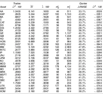
ofλ.The estimates are based on high-frequency stock returns of Alcoa (left panels) and Microsoft (right panels) in year the 2000. The details about the estimation ofλare deferred to Sec-tion 5. The upper panels presentr0(λ,ˆ m)andr1(λ,ˆ m), where r1(λ,ˆ m) identify their respective optimal sampling
frequen-cies, m∗0 and m∗1. For the AA returns, we find that the opti-mal sampling frequencies are m∗0,AA=44 and m∗1,AA=511 (corresponding to intraday returns spanning 9 minutes and 46 seconds) and that the theoretical reduction of the RMSE is 33.1%. The curvatures of r0(λ,ˆ m)andr1(λ,ˆ m)in the
neigh-borhood ofm∗0 andm∗1 show thatRV(ACm)
1 is less sensitive than
RV(m)to the choice ofm.
The middle panels of Figure 3 display the relative RMSE of
RV(ACm)
1to that of (the optimal)RV
(m∗0)and the relative RMSE of
RV(m) to that of (the optimal)RV(m∗1)
AC1. These panels show that the RV(ACm)
1 continues to dominate the “optimal” RV
(m∗0) for a wide ranges of frequencies, not just in a small neighborhood of the optimal value,m∗1. This robustness ofRVAC1 is quite use-ful in practice, where λ and (hence) m∗1 are not known with certainty. The result shows that a reasonably precise estimate
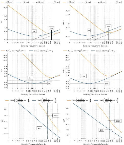
Figure 3. RMSE Properties of RV and RVAC
1Under Independent Market Microstructure Noise Using Empirical Estimates ofλfor 2000. The
up-per panels display the RMSEs for RV and RVAC1using estimates ofλ, r0(λ, m) and rˆ 1(λ, m), and the corresponding RMSEs in the absence of noise,ˆ
r0(0, m) and r1(0, m). The middle panels are the relative RMSEs of RV(m)and RV(m)AC1to RV (m∗
0)and RV(m∗1)
AC1, as defined by r0(λ, m)/rˆ 1(λ, mˆ ∗1) and
r1(λ, m)/rˆ 0(λ, mˆ ∗
0). The lower panels show the percentage increase in the RMSE for different sampling frequencies caused by market microstructure
noise. The x -axis gives the sampling frequency of intraday returns as defined byδi,m=(b−a)/m in units of seconds, where b−a=6.5 hours
(a trading day).
ofλ(and hencem∗1)will lead to aRVAC1 that dominates RV. This result is not surprising, because recent developments in this literature have shown that it is possible to construct kernel-based estimators that are even more accurate thanRVAC1 (see Barndorff-Nielsen et al. 2004; Zhang 2004).
A second, very interesting aspect that can be analyzed based on the results of Corollary 2 is the accuracy of theoretical re-sults derived under the assumption thatλ=0 (no market mi-crostructure noise). For example, the accuracy of a confidence interval for IV, which is based on asymptotic results that ignore
the presence of noise, will depend on λ and m. The
expres-sions of Corollary 2 provide a simple way to quantify the the-oretical accuracy of such confidence intervals, including those of Barndorff-Nielsen and Shephard (2002). Figure 3 provides valuable information on this question. The upper panels of Fig-ure 3 present the RMSEs of RV(m) and RV(ACm)
ture noise are pronounced at the higher sampling frequencies. The lower panels of Figure 3 quantify the discrepancy between the two “types” of RMSEs as a function of the sampling fre-quency. These plots present 100[r0(λ,ˆ m)−r0(0,m)]/r0(0,m)
and 100[r1(λ,ˆ m)−r1(0,m)]/r1(0,m)as a function ofm. Thus
the former reveals the percentage increase of the RV’s RMSE due to market microstructure noise, and the second line simi-larly shows the increase of theRVAC1’s RMSE due to noise. The increase in the RMSE may be translated into a widening of a confidence intervals for IV (aboutRV(m)orRV(ACm)
1). The ver-tical lines in the right panels mark the sampling frequency cor-responding to 5-minute sampling under CTS and show that the “actual” confidence interval (based onRV(m)) is 105.94% larger than the “no-noise” confidence interval for AA, whereas the en-largement is 22.37% for MSFT. At 20-minute sampling, the dis-crepancy is less than a couple of percent, so in this case the size distortion from being oblivious to market microstructure noise is quite small. The corresponding increases in the RMSE ofRV(ACm)
1 are 9.41% and 3.07%. Thus a “no-noise” confidence interval aboutRV(ACm)
1 is more reliable than that aboutRV (m) at
moderate sampling frequencies. Here we have used an estima-tor ofλbased on data from the year 2000, before the tick size was reduced to 1 cent. In our empirical analysis we find the noise to be much smaller in recent years, such that “no-noise approximations” are likely to be more accurate after decimal-ization of the tick size.
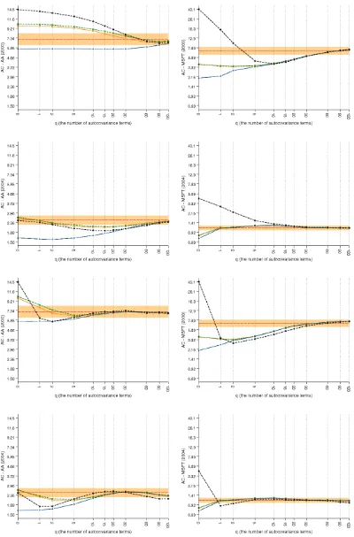
Figure 4 presents the volatility signature plots for RV(ACm)
1, where we have used the same scale as in Figure 1. When sam-pling in calender time (the four upper panels), we see a pro-nounced bias inRV(ACm)
1when intraday returns are sampled more frequently than every 30 seconds. The main explanation for this is that CTS will sample the same price multiple times whenmis large, which induces (artificial) autocorrelation in intraday re-turns. Thus, when intraday returns are based on CTS, it is nec-essary to incorporate higher-order autocovariances ofyi,mwhen mbecomes large. The plots in rows 3 and 4 are signature plots when intraday returns are sampled in tick time. These also re-veal a bias inRV(ACxtick)
1 at the highest frequencies, which shows that the noise is time dependent in tick time. For example, the
MSFT 2000 plot suggests that the time dependence lasts for 30 ticks, perhaps longer.
Fact II. The noise is autocorrelated.
We provide additional evidence of this fact, based on other empirical quantities, in the following sections.
4. THE CASE WITH DEPENDENT NOISE
In this section we consider the case where the noise is time-dependent and possibly correlated with the efficient re-turns, y∗i,m. Following earlier versions of the present article, issues related to time dependence and noise–price correlation have been addressed by others, including Aït-Sahalia et al. (2005b), Frijns and Lehnert (2004), and Zhang (2004). The time scale of the dependence in the noise plays a role in the asymp-totic analysis. Although the “clock” at which the memory in the noise decays can follow any time scale, it seems reasonable for it to be tied to calendar time, tick time, or a combination of the two. We first consider a situation where the time dependence is specific to calendar time, then consider the case with time dependence in tick time.
4.1 Dependence in Calender Time
To bias-correct the RV under the general time-dependent type of noise, we make the following assumption about the time dependence in the noise process.
Assumption 4. The noise process has finite dependence in the sense thatπ(s)=0 for alls> θ0for some finiteθ0≥0, and E[u(t)|p∗(s)] =0 for all|t−s|> θ0.
The assumption is trivially satisfied under the independent noise assumption used in Section 3. A more interesting class of noise processes with finite dependence are those of the mov-ing average type, u(t)=tt−θ
0ψ (t−s)dB(s), whereB(s)
rep-resents a standard Brownian motion and ψ (s) is a bounded
(nonrandom) function on [0, θ0]. The autocorrelation function
for a process of this kind is given byπ(s)=sθ0ψ (t)ψ (t−s)dt, fors∈ [0, θ0].
Theorem 2. Suppose that Assumptions 1, 2, and 4 hold and letqmbe such thatqm/m> θ0. Then (under CTS),
qm is that it may produce a negative estimate of volatility, because the covariances are not scaled downward in a way that would guarantee positivity. This is par-ticularly relevant in the situation where intraday returns have a “sharp negative autocorrelation” (see West 1997), which has been observed in high-frequency intraday returns constructed from transaction prices. To rule out the possibility of a negative estimate, one could use a different kernel, such as the Bartlett kernel. Although a different kernel may not be entirely
Figure 4. Volatility Signature Plots for RVAC1 Based on Ask Quotes ( ), Bid Quotes ( ), Mid-Quotes ( ), and Transaction Prices ( ). The left column is for AA and the right column is for MSFT. The two top rows are based on calendar time sampling; the bot-tom rows are based on tick time sampling. The results for 2000 are the panels in rows 1 and 3, and those for 2004 are in rows 2 and 4. The horizontal line represents an estimate of the average IV,σ¯2≡RV(1 tick)ACNW
30, that is defined in Section 4.2. The shaded area aboutσ¯
2represents an
approximate 95% confidence interval for the average volatility.
ased, it may result is a smaller MSE than that ofRVAC.
Inter-estingly, Barndorff-Nielsen et al. (2004) have shown that the subsample estimator of Zhang et al. (2005) is almost identical to the Bartlett kernel estimator.
In the time series literature, the lag length,qm, is typically
chosen such thatqm/m→0 as m→ ∞, for example, qm =
⌈4(m/100)2/9⌉,where⌈x⌉denotes the smallest integer that is greater than or equal to x. But if the noise were dependent in calendar time, then this would be inappropriate, because it would lead toqm=3 when a typical trading day (390 minutes)
were divided into 78 intraday returns (5-minute returns) and to qm =6 if the day were divided into 780 intraday returns
(30-second returns). So the formerq would cover 15 minutes, whereas the latter would cover 3 minutes (6×30 seconds), and
in fact the period would shrink to 0 as m→ ∞. Under
As-sumptions 2 and 4, the autocorrelation in intraday returns is specific to a period in calendar time, which does not depend onm; thus it is more appropriate to keep the width of the “au-tocorrelation window,”qm/m, constant. This also makesRV(ACm)
more comparable across different frequencies,m. Thus we set
qm= ⌈(b−wa)/m⌉,wherewis the desired width of the lag
win-dow andb−a is the length of the sampling period (both in
units of time), such that(b−a)/m is the period covered by each intraday return. In this case we writeRV(ACm)
w in place of
RV(ACm)
qm. Therefore, if we were to sample in calendar time and
setw=15 min andb−a=390 min, then we would include
qm= ⌈m/26⌉autocovariance terms.
When qm is such that qm/m> θ0≥ 0, this implies that RV(ACm)
qm cannot be consistent for IV. This property is common for estimators of the long-run variance in the time series liter-ature wheneverqm/mdoes not converge to 0 sufficiently fast
(see, e.g., Kiefer, Vogelsang, and Bunzel 2000; and Jansson 2004). The lack of consistency in the present context can be un-derstood without consideration of market microstructure noise. In the absence of noise, we have that var(y2i,m)=2σi4,m and
under CTS. This shows that the variance does not vanish when
qmis such thatqm/m> θ0>0.
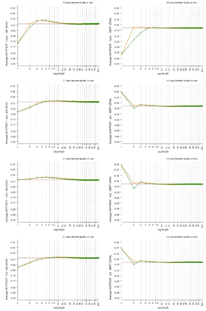
The upper four panels of Figure 5 represent a new type of signature plots forRV(AC1 sec)
q . Here we sample intraday returns
every second using the previous-tick method and now plot q
along thex-axis. Thus these signature plots provide informa-tion on time dependence in the noise process. The fact that the
RV(AC1 sec)
q of the four price series differ and have not leveled off is evidence of time dependence. Thus in the upper four panels, where we sample in calendar time, it appears that the depen-dence lasts for as long as 2 minutes (AA, year 2000) or as short
as 15 seconds (MSFT, year 2004). We comment on the lower four panels in the next section, where we discuss intraday re-turns sampled in tick time.
4.2 Time Dependence in Tick Time
When sampling at ultra-high frequencies, we find it more nat-ural to sample in tick time, such that the same observation is not sampled multiple times. Furthermore, the time dependence in the noise process may be in tick time rather than calender time. Several results of Bandi and Russell (2005) allow for time de-pendence in tick time (while the price–noise correlation is as-sumed away).
The following example gives a situation with market mi-crostructure noise that is time-dependent in tick time and corre-lated with efficient returns.
Example 1. Let t0<t1<· · ·<tm be the times at which
prices are observed, and consider the case where we sample in-traday returns at the highest possible frequency in tick time. We suppress the subscriptmto simplify the notation. Suppose that the noise is given byui=αy∗i +εi, whereεiis a sequence of iid
random variables with mean 0 and variance var(εi)=ω2. Thus α=0 corresponds to the case with independent noise assump-tion, andα=ω2=0 corresponds to the case without noise. It
1 is almost unbiased for the IV.
In this simple example,uiis only contemporaneously
corre-lated withy∗i. In practice, it is plausible thatui could also be
correlated with lagged values ofy∗i, which would yield a more complicated time dependence in tick time. In this situation we could use RV(AC1 tick)
q , with aq sufficiently large to capture the time dependence.
Assumption 4 and Theorem 2 are formulated for the case with CTS, but a similar estimator can be defined under depen-dence in tick time. The lower four panels of Figure 5 are the
Figure 5. Volatility Signature Plots of RVAC(1 sec)
q (four upper panels) and RV
(1 tick)
ACq (four lower panels) for Each of the Price Series: Ask
Quotes ( ), Bid Quotes ( ), Mid-Quotes ( ), and Transaction Prices ( ). The x -axis is the number of autocovariance terms, q, included in RVAC(1 sec)
q . The left column is for AA, and the right column is for MSFT. The results for 2000 are the panels in rows 1 and 3, and those
for 2004 are in rows 2 and 4. The horizontal line represents an estimate of the average IV,σ¯2≡RV(1 tick)ACNW
30, that is defined in Section 4.2. The
shaded area aboutσ¯2represents an approximate 95% confidence interval for the average volatility.
signature plots for RV(AC1 tick)
q , whereq is the number of
auto-covariances used to bias correct the standard RV. From these plots, we see that a correction for the first couple of autoco-variances has a substantial impact on the estimator, but higher-order autocovariances are also important, because the volatility signature plots do not stabilize untilq≥30 in some cases (e.g., MSFT in 2000). This time dependence was longer than we had anticipated; thus we examined whether a few “unusual” days were responsible for this result. However, the upward-sloping volatility signature (untilqis about 30) is actually found in most daily plots ofRV(AC1 tick)
q againstqfor MSFT in the year 2000.
In Section 3 we analyzed the simple kernel estimator that incorporates only the first-order autocovariance of intraday re-turns, which we now generalize by including higher-order auto-covariances. We did this to make the estimator,RV(AC1 tick)
q , robust to both time dependence in the noise and correlation between noise and efficient returns. Interestingly, Zhou (1996) also pro-posed a subsample version of this estimator, although he did not refer to it as a subsample estimator. As is the case forRV(AC1 tick)
q ,
this estimator is robust to time dependence that is finite in tick time. Next, we describe the subsample-based version of Zhou’s estimator.
Lett0<t1<· · ·<tN be the times at which prices are
ob-served in the interval [a,b], where a=t0 and b=tN. Here mneed not be equal toN(unlike the situation in the previous ex-ample), because we use intraday returns that span several price observations. We use the following notation for such (skip-k) intraday returns:
(assuming that N/k is an integer), which is a sum involving
m=N/k terms. The subsample version RV(ACm)
1, proposed by Zhou (1996), can be expressed as
1
show that this subsample estimator is approximately given by
RV(ACNW1 tick)
Thus this estimator equals theRV(AC1 tick)
k plus an additional term, a Bartlett-type weighted sum of higher-order covariances. In-terestingly, Zhou (1996) showed that the subsample version of his estimator [see (6)] has a variance that is (at most) of order
O(Nk)+O(1k)+O(N
k2)(assuming constant volatility). This term is of orderO(N−1/3)ifkis chosen to be proportional toN2/3, as was done by Zhang et al. (2005). It appears that Zhou may have consideredkas fixed in his asymptotic analysis, because he referred to this estimator as being inconsistent (see Zhou 1998, p. 114). Therefore, the great virtues of subsample-based estimators in this context were first recognized by Zhang et al. (2005).
5. EMPIRICAL ANALYSIS
We now analyze stock returns for the 30 equities of the DJIA. The sample period spans 5 years, from January 3, 2000 to De-cember 31, 2004. We report results for each of the years indi-vidually, but give some of the more detailed results only for the years 2000 and 2004 to conserve space. The tick size was re-duced from 1/16 of 1 dollar to 1 cent on January 29, 2001, and to avoid mixing mix days with different tick sizes, we drop most of the days during January 2001 from our sample. The data are transaction prices and quotations from NYSE and NASDAQ, and all data were extracted from the Trade and Quote (TAQ) database.
We filtered the raw data for outliers, and discarded
transac-tions outside the period 9:30 AM–4:00 PM and removed days
with less than 5 hours of trading from the sample. This reduced the sample to the number of days reported in the last column of Table 1. The filtering procedure removed obvious data errors, such as zero prices. We also removed transaction prices that were more than one spread away from the bid and ask quotes. (Details of the filtering procedure are described in a techni-cal appendix available at our website.) The average number of transactions/quotations per day are given for each year in our sample; these reveal a steady increase in the number of trans-actions and quotations over the 5-year period. The numbers in parentheses are the percentages of transaction prices that dif-fer from the proceeding transaction price and similarly for the quoted prices. The same price is often observed in several con-secutive transactions/quotations, because a large trade may be divided into smaller transactions, and a “new” quote may sim-ply reflect a revision of the “depth” while the bid and ask prices remain unchanged. We use all price observations in our analy-sis. Censoring all of the zero intraday returns does not affect the RV, but has an impact on the autocorrelation of intraday returns.
Our analysis of quotation data is based on bid and ask prices and the average of these (mid-quotes). The RVs are cal-culated for the hours that the market is open, approximately 390 minutes per day (6.5 hours for most days). Our tables present results for all 30 equities, whereas our figures present
142
Jour
nal
of
Business
&
Economic
Statistics
,
A
pr
il
2006
Table 1. Equity Data: Summary Statistics
Transactions/day Quotes/day
No. of days
Symbol Name Exchange 2000 2001 2002 2003 2004 2000 2001 2002 2003 2004
AA Alcoa NYSE 997(41) 1,479(50) 1,898(50) 2,153(45) 3,150(43) 1,384(33) 1,875(44) 2,775(38) 5,309(32) 7,560(34) 1,223 AXP American Express NYSE 1,584(45) 2,449(54) 2,791(53) 3,371(52) 2,752(44) 2,004(42) 3,123(46) 3,745(41) 7,293(43) 7,464(34) 1,221 BA Boeing Company NYSE 1,052(39) 1,730(49) 2,306(52) 2,961(48) 3,037(47) 1,587(30) 2,492(46) 3,552(43) 6,475(42) 8,022(39) 1,221 C Citigroup NYSE 2,597(44) 3,129(51) 3,997(49) 4,424(46) 4,803(47) 3,076(27) 3,994(42) 5,039(40) 7,993(37) 9,316(37) 1,221 CAT Caterpillar Inc. NYSE 747(40) 1,260(50) 1,673(53) 2,414(54) 3,154(56) 1,039(33) 2,002(43) 2,879(40) 5,852(46) 8,185(51) 1,221 DD Du Pont De Nemours NYSE 1,257(48) 1,853(54) 2,100(53) 2,963(51) 3,077(49) 1,858(30) 2,915(43) 3,418(39) 6,663(41) 8,069(38) 1,220 DIS Walt Disney NYSE 1,304(39) 2,013(53) 2,882(54) 3,448(48) 3,564(46) 1,525(25) 2,893(43) 4,750(36) 7,768(33) 8,480(34) 1,221 EK Eastman Kodak NYSE 775(42) 1,128(50) 1,392(45) 2,008(45) 1,941(44) 1,181(35) 1,941(44) 2,322(37) 4,910(35) 5,715(31) 1,220 GE General Electric NYSE 3,191(41) 3,157(52) 4,712(54) 4,828(48) 4,771(44) 2,888(34) 3,646(48) 5,559(42) 8,369(31) 10,051(24) 1,221 GM General Motors NYSE 988(37) 1,357(50) 2,448(49) 2,874(49) 2,855(47) 1,572(35) 2,009(44) 4,246(37) 6,262(35) 6,889(34) 1,221 HD Home Depot Inc. NYSE 1,961(42) 2,648(51) 3,533(52) 3,843(49) 3,642(46) 2,161(31) 2,946(51) 4,181(42) 7,246(36) 8,005(31) 1,221 HON Honeywell NYSE 1,122(38) 1,453(52) 1,872(47) 2,482(47) 2,668(47) 1,378(33) 2,364(47) 3,120(40) 5,385(40) 6,542(39) 1,221 HPQ Hewlett–Packard NYSE 1,900(46) 2,321(51) 2,543(46) 3,263(43) 3,708(43) 2,394(45) 3,170(43) 3,226(36) 6,536(31) 8,700(27) 1,218 IBM Int. Business Machines NYSE 2,322(55) 3,637(63) 3,492(61) 4,111(60) 4,553(55) 3,319(53) 4,729(55) 6,688(37) 7,790(49) 9,447(51) 1,220 INTC Intel. Corp. NASD 14,982(73) 15,637(83) 15,194(80) 10,918(71) 9,078(67) 10,599(17) 12,512(32) 17,622(45) 19,554(39) 19,828(42) 1,230 IP International Paper NYSE 1,002(40) 1,509(50) 1,971(50) 2,569(47) 2,283(44) 1,368(31) 2,346(41) 3,134(37) 5,997(40) 6,417(34) 1,221 JNJ Johnson & Johnson NYSE 1,492(49) 2,059(57) 2,541(60) 3,272(53) 3,853(48) 1,739(36) 2,322(47) 3,091(42) 6,529(39) 8,687(36) 1,221 JPM J. P. Morgan NYSE 1,317(52) 2,555(51) 2,973(52) 3,836(49) 3,939(46) 1,839(52) 3,384(46) 4,079(39) 7,387(36) 8,808(30) 1,221 KO Coca-Cola NYSE 1,376(45) 1,662(51) 2,349(52) 2,854(50) 3,320(48) 1,635(32) 2,063(48) 3,221(42) 6,240(39) 7,498(35) 1,221 MCD McDonalds NYSE 1,109(39) 1,779(50) 2,226(49) 2,638(45) 2,790(43) 1,578(21) 2,334(42) 3,065(37) 5,763(33) 7,331(31) 1,221 MMM Minnesota Mng. Mfg. NYSE 868(44) 1,563(56) 2,054(57) 3,092(58) 3,370(48) 1,157(45) 2,462(50) 3,253(48) 7,100(52) 8,228(46) 1,220 MO Philip Morris NYSE 1,283(38) 1,942(53) 3,047(54) 3,473(50) 3,404(48) 2,365(13) 3,266(34) 4,174(40) 6,776(38) 7,721(38) 1,220 MRK Merck NYSE 1,832(41) 1,943(51) 2,574(52) 3,639(50) 3,663(45) 2,021(35) 2,381(48) 3,262(41) 6,927(43) 7,658(34) 1,221 MSFT Microsoft NASD 13,900(68) 14,479(86) 15,257(85) 12,013(73) 8,643(66) 8,275(14) 13,341(40) 18,234(66) 19,833(45) 19,669(41) 1,229 PG Procter & Gamble NYSE 1,518(44) 1,881(54) 2,631(52) 3,314(52) 3,668(50) 2,584(27) 3,137(43) 4,555(42) 7,535(47) 8,397(45) 1,221 SBC Sbc Communications NYSE 1,603(37) 2,267(52) 3,038(52) 3,060(46) 3,364(43) 2,042(24) 2,791(48) 3,909(39) 6,478(31) 8,346(26) 1,220 T AT&T Corp. NYSE 2,233(29) 1,851(40) 2,224(43) 2,353(44) 2,412(39) 1,657(26) 2,238(40) 2,931(32) 5,307(30) 7,091(20) 1,221 UTX United Technologies NYSE 767(41) 1,354(51) 1,986(53) 2,758(55) 3,107(55) 1,111(46) 2,183(46) 3,075(45) 6,657(49) 7,996(53) 1,220 WMT Wal-Mart Stores NYSE 1,946(43) 2,368(54) 2,847(58) 2,860(51) 4,394(50) 2,609(27) 2,675(47) 3,971(44) 5,610(39) 8,744(40) 1,221 XOM Exxon Mobil NYSE 1,720(41) 2,227(53) 3,467(54) 4,198(48) 4,489(47) 1,979(33) 2,712(43) 4,677(37) 8,340(32) 9,950(29) 1,219