www.elsevier.nl / locate / econbase
Privatisation and market structure in a transition
economy
a,* b
John Bennett , James Maw a
Department of Economics and Finance, Brunel University, Uxbridge, Middlesex, UB8 3PH, UK b
Department of Economics, University of Wales, Swansea, SA2 8PP, UK
Received 1 August 1997; received in revised form 1 December 1998; accepted 1 October 1999
Abstract
A model is developed in which an industry of N$1 firms is privatised. The ‘participation’ method of privatisation is used, whereby firms are sold for cash, but the state retains a proportionate share of ownership. In each firm the new private owner has the opportunity to make a reorganisational investment, before output is produced. This investment is unobservable by the state, and therefore non-contractible. There is Cournot competition in the product market. The welfare-maximising retained ownership share for the state is analysed, taking into account that potential buyers of firms may have limited access to finance. 2000 Elsevier Science S.A. All rights reserved.
Keywords: Privatisation; Transition economy; Market structure
JEL classification: L33; P21
1. Introduction
In the transition economies of Central and Eastern Europe and the former Soviet Union privatisation has taken place by a variety of methods (see, for example, Estrin, 1994; Brada, 1996). Following the lead of the Czech Republic and Russia, the most common method (used or proposed) has been voucher, or mass,
*Corresponding author.
E-mail address: [email protected] (J. Bennett)
privatisation. However, Germany, Hungary and Estonia have relied heavily on privatisation by sale, with foreign investors playing a major role in the latter two countries. Moreover, from 1995 onwards the Czech and Slovak Republics, Russia and several other countries switched emphasis to privatisation by sale (EBRD, 1996b). In many of these privatisations the state has kept a significant share in the ownership of firms, while giving up all managerial control (see Perotti, 1995, on the Hungarian case). This ‘participation’ model of sale, which is the subject of the present paper, has been forcefully advocated by Sinn and Sinn (1993) and Bolton and Roland (1992). It has also been analysed formally by Demougin and Sinn (1994), on whose work we build. In this model, privatisation is undertaken with two objectives in mind: to bring about investment in the modernisation of firms
1
and to generate revenue for the state. The investment is required because of decades of poor technological and organisational achievement under Communism, while state revenue is a critical factor largely because profit tax revenue has collapsed at the same time as some spending needs (for example, for the provision
2
of a social safety net) have risen substantially.
Unlike Demougin and Sinn, who focus on risk-sharing, we do not allow for uncertainty. This simplification allows us to introduce several other considerations into the analysis. First, in previous theoretical work it does not seem to have been taken into account that the firms being sold may compete against one another in the product market. Yet, both the amount that a buyer is willing to pay for a firm and the willingness of the buyer then to invest in the reorganisation of the firm will depend on how competitive the product market is. In our model this is recognized
by supposing that an industry of N firms is being privatised, where N$1. The
buyer of each firm is assumed to make an investment in its reorganisation before production takes place, after which firms play a Cournot production game.
Second, we assume that investment by the new private owner of a firm involves the allocation of resources in a way that may be unobservable and non-contract-ible. In contrast, Demougin and Sinn assume for most of their analysis that there is contractibility, with the amount of investment the buyer will make specified in the contract when the firm is bought. This corresponds to the investment targets that were set for buyers of German SOEs and which have more recently been specified in Estonia and the Slovak Republic (EBRD, 1996b). However, as Demougin and Sinn point out, a government will be unable to observe the real cost to a company of transferring managerial know-how to an acquired firm, for this depends on the managers’ alternative occupations. In our model the amount of investment is chosen freely by the buyer and may not be observable to outsiders. Hence, we
1
A major economic objective of privatisation that we do not consider is change in corporate governance and / or managerial motivation. Also, we ignore political objectives such as to make the reform process irreversible. See Estrin (1994) and Dewatripont and Roland (1996).
2
3
suppose that the full cost of investment is borne by the buyer. The government’s participation in the firm relates only to the share it takes of production profit (the government is a sleeping partner). This participation may be interpreted as ownership or as a cash-flow tax. A cash flow-tax may be less open to abuse than a
4
profit tax would be.
Third, we investigate two different forms of reorganisational investment. One form updates methods, reducing marginal cost for a good that is already in production. The other form creates capacity to produce a new output, for example, as Volkswagen has created capacity in Skoda to produce cars of, for Skoda, a previously unachieved quality. For the latter form of investment we also allow for the possibility that the good is internationally traded, with producers facing a horizontal demand curve.
Fourth, we allow for the possibility that any potential buyer of a firm may be financially constrained. This is to reflect the fact that in transition economies the main source of investment funds, domestic savings, has declined sharply in real terms, while the fragility of the banking sector undermines savings mobilisation and financial intermediation. Although there has been a recent increase in sales of firms to foreign companies, this has been concentrated in a few of the transition economies and in particular market segments (EBRD, 1996b). Furthermore,
5
foreign companies also have limits on the funds they have available. In our model the finance constraint plays two potential roles. It may prevent a buyer from paying the amount the firm is worth; and given the amount it pays for the firm, the buyer may have insufficient access to funds to raise the amount of reorganisation investment to the profit-maximising level.
We begin our analysis by formulating a ‘basic model’ in which there is no binding constraint on finance. Given that the industry faces a downward-sloping demand curve, then, if government revenue is given a large enough weight in the welfare function, the optimum retained ownership share for the state tends to be larger when there are more firms in the industry being privatised. This conclusion is unaffected by whether reorganisational investment occurs as cost reduction or capacity expansion. However, for the latter case, we also allow for the effect of international trade through the alternative assumption that the goods demand curve is horizontal. Then, we find that, provided the industry is commercially viable, the state should not keep any share in ownership. When we introduce a binding limit on finance into the model, we find that, generally speaking, the more finance is
3
In Section 3.3 of the paper we discuss whether, when investment is contractible, it is nonetheless desirable to make the buyer bear its full cost.
4
It would be possible to combine the two interpretations of the government’s share, for example, with a uniform cash-flow tax imposed on all industries, together with a government ownership share that varies across industries.
5
limited, the greater is the share in ownership that the state should keep. Also, for the case of investment in capacity expansion we describe a possible situation in which a limit on finance leads to the non-existence of an equilibrium price for a firm.
Since we assume throughout that any retained ownership in a firm by the state is in the form of non-voting shares, the government cannot control a firm’s behaviour directly. Nonetheless, the government can influence a firm’s behaviour through its choice of how big an ownership share to keep. The underlying feature of the model that generates our main results is the tendency, when finance is unlimited, of Cournot competitors to overinvest relative to the collusive profit-maximising solution. When, however, the government takes a share of production profit, the incentive to invest is less for the private owner, ceteris paribus. This can raise production profit for the industry and revenue for the government (from its ownership share, if any, plus the price it is able to get for the share it sells). The government should take an ownership share if it values revenue sufficiently greatly, compared with investment (or consumer surplus). If a limit on finance for firms prevents such a solution from being attained, the optimal government ownership share tends to be yet higher because this causes the price that a private buyer is willing to pay for its share of a firm to be lower. The private buyer is therefore left with a larger proportion of its financial resources to use for investment, limiting the fall of investment below the level in the finance-unconstrained solution.
If there were no binding constraints on the availability of finance or on the value that the private ownership share could take, a first-best solution would always be achieved. However, when such constraints bind we enter a second-best world. A constraint that we impose throughout is that the private ownership share cannot exceed unity, i.e. the state will not subsidise production profit. This constraint binds when the government values investment greatly compared to revenue. Another potentially binding constraint, the effects of which we note in the final section, is that for ‘privatisation’ to take place the private ownership share may have to be at least one-half.
Before proceeding, it is worth considering the possible empirical relevance of the potential for overinvestment when oligopolies are privatised, though we can only draw indirect inferences. First, note that, according to EBRD (1995), the ratio of gross fixed investment to GDP for 1993–1994 was ‘fairly high’ in many transition economies, compared to the OECD average (for 1994) of 20.6%. For example, for the Czech and Slovak Republics, Slovenia, Hungary, Estonia, Lithuania, Belarus and Russia the ratio was in the range 20–28%. And EBRD (1996a) reports that the ratio of investment to GDP tended to rise from 1994
6
onwards outside the CIS. It should also be emphasized that much investment is in
6
forms that are not recorded in official statistics. For example, as we have already mentioned, there is an opportunity cost to transferring managerial resources from
7
the other activities of a company. This may be especially important for foreign investors. Second, we may focus on Hungary and Estonia, since, apart from the special case of Germany, these are the main exponents of privatisation by direct sale. Duponcel (1998) reports that in the Hungarian and Estonian food sectors foreign direct investment has considerably increased competition, while EBRD (1997) notes that in Estonia the contractual investment obligations specified by the government when selling firms have often been exceeded, sometimes by a wide margin. Though such evidence is only circumstantial, it is consistent with the hypothesis that investment in some industries may be greater than the amount that would maximise government revenue.
We begin our analysis by examining the ‘basic’ case, in which finance is unconstrained. The model is set up for this case in Section 2 and solved in Section 3. Then, in Section 4, we introduce a shortage of finance. Section 5 concludes by discussing the implications of changing our set of assumptions. Appendix A provides proofs of propositions and deals with the technical points.
2. The basic model
There are N$1 firms in an industry producing a homogeneous good. All the
firms are state-owned; there is no production of the good by the de novo sector and no foreign trade in the good. The firms may have been subject to some limited
8
restructuring. They are simultaneously sold into the private sector, where the
9
number of potential buyers is large relative to N. The timing of the model is as follows.
• Decision Stage: The government specifies the share 12s that it will take from
7
Also, particularly in the case of Russia a significant proportion of investment is ‘informal’ (Linz and Krueger, 1998) or ‘relational’ (Gaddy and Ickes, 1998) and so does not show up in data.
8
Grosfeld and Roland (1995) distinguish ‘defensive’ restructuring, which is restricted to labour-shedding and downsizing activities, from ‘strategic’ restructuring, which involves thoughtful business projects and modernisation investments. In practice SOEs have engaged primarily in defensive restructuring. The reorganisation investment that occurs after privatisation in our model may be regarded as strategic.
9
the profits earned by the firms in the production stage.
• Sales Stage: The government then sells each firm for a cash price P and a share
10
12s. Given s, competitive bidding for each firm determines P.
• Investment Stage: The buyer of any firm j then invests a non-negative amount ij
( j51,2, . . . ,N ).
• Production Stage: Finally, the firms play a Cournot production game. Each firm j produces output q .j
Once the firms are sold, the state takes no part in investment or production decisions. Investment is likely to be multi-dimensional, making the writing of a complete contract extremely costly and difficult to enforce. We therefore assume that investment by the new private owner (for short, ‘the owner’) is non-contractible. Nonetheless, the government can affect investment through its choice
11
of s. We restrict this choice to the range s[(0,1], though for analytical purposes we shall also consider values of s outside this range.
We shall henceforth omit firm subscripts, because we shall be considering only
12
symmetric equilibria. At the production stage the industry faces the demand
curve:
p5A2bNq, A.0, b$0 (1)
where p is the unit price of the good and A and b are constants. Firms play a Cournot game at this stage, with each one generating a gross production profitP. The characterization of this game depends on the form that the reorganisation investment takes. We shall return to this below.
10
We do not allow for discounting and we assume that no output is produced until the production stage. These simplifications do not have significant qualitative effects on the results.
11
Suppose 12s is an ownership share (not a tax rate). An objection that might then be made to our
formulation is that the new private owner of the firm could dilute the government’s share, ex post, by issuing further shares, thereby making meaningless the government’s ‘optimum’ choice of s. However, if the private owner behaved in this way, the government could respond by imposing a profit tax that restores the share of profit it receives to the optimum level. By the same token, it might be objected that the government could in any case impose a profit tax, ex post (after privatisation) of any size, so that the choice of the value of s analysed in this paper is of no significance. However, the government might wish to avoid such behaviour because it would send an adverse signal to potential buyers of firms in other industries yet to be privatised, thereby damaging the government’s future revenue prospects. We disregard such complications and assume that s is fixed once-and-for-all at the decision stage.
12
Denote the net profit accruing to the owner of a firm, for the investment and production stages combined, by:
p 5sP 2i (2)
For any given level of i by a firm, the resulting level of its p depends on the
amount of investment by other firms. Given s, the owner of each firm chooses i to
maximise p, treating investment by other firms as constant. Denote the firm’s
investment in the resulting Nash equilibrium by i*(s) and the corresponding value
of p byp*(s). Competition between the potential buyers forces the price P paid
for a firm up to the level at which it squeezes out all rent for the new owner:
P5p*(s) (3)
Going back to the decision stage, the government chooses s optimally, taking into account behaviour in the three succeeding stages. It wishes to maximise the concave welfare function:
w5W(R, CS ) (4)
where government revenue R is given by:
R5N Pf 1(12s)Pg (5)
and CS is consumer surplus, which, using (1), is given by:
2
CS5b Nq / 2s d (6)
Since CS is increasing in i in the model, (4) is equivalent to w5W(R, i ). We do
not include profit as a separate argument of W because, in the solution to the
model, p accrues to the government as the price P paid for the firm and so is
already taken into account through the appearance of R in (4).
Finally, we distinguish two cases, corresponding to the two forms that reorganisational investment may take. First, suppose investment is in cost reduction (Case CR). In this case, we assume that, given the amount of investment
i by a firm, it has a constant unit cost of goods production c, where:
c5C(i ), C9(i ),0, C0(i ).0 (7)
¯ ¯
We write C(0);C and assume that A.C.0. Given i, the equilibrium of the
ensuing Cournot production game yields:
2
q5hA2C i(s) /b(Nf gj 11), P 5bq (8)
Alternatively, investment may be in capacity expansion (Case CE):
¯q5Q(i ), Q9(i ).0, Q0(i ),0 (9)
¯
constant and the same for all firms (c,A). In the solution, each firm will only
install capacity that will be fully used in the production stage. Analytically, the investment and production stages therefore collapse into one stage. For each firm:
q5Q i(s) ,f g P 5hA2bNQ i(s)f g2c Q i(s)j f g (10) In the Nash equilibrium each firm sets i5i*(s) to maximise (2) subject to (10). As
a subcase, we can accommodate the assumption of free international trade in the
good at the given unit price by supposing that b50. Then, from (1) and (10),
13
p5A and P 5(A2c)Q i*(s) .f g
3. Solution of the basic model
3.1. Investment in cost reduction (CR)
First, we assume that there is no limit on the availability of finance F and that investment is in cost reduction. Taking into account that production will be a Cournot game, as represented by Eq. (8), we begin by considering the investment stage. Here, we can disregard the price P paid for the firm because this is a by-gone. In the Nash equilibrium, with i chosen to maximisep, as defined by (2), the f.o.c. for an internal solution is:
2 2b(N11)
]]]]
A2C(i*) C9(i*)5 (11)
f g 2Ns
We assume throughout that for all i$0
2
f;fA2C(i ) Cg 0(i )2fC9(i )g .0 (12)
2 2
This ensures that d p/ di ,0, so that thep-maximum is unique.
Firms will invest if the private ownership parameter s is sufficiently large. It is
shown in Appendix A that i*.0 if s.s , where:0
2 2b(N11)
]]]]]
s05 ¯ (13)
2NC9(0) A
s
2Cd
If, however, s#s , firms set i*0 50. From (11) it is found that:
2 A2C(i*) C9(i*) /sf .0 for s.s
di* f g 0
] 5
H
(14)ds 0 for s#s0
Thus, if the share of production profit P going to the owner of the firm is large
13
enough to induce positive investment, a higher share induces more investment. Also, note from (11) that i* is decreasing in N for s.s .0
We now go back to the decision stage. In choosing s the government takes into account what will happen in the three succeeding stages. We assume first that the government chooses s to maximise revenue.
Proposition 1. When investment is in cost reduction, revenue R is maximized by
˜ setting s5s :R
˜
(i ) sR51 /N if s0,1 /N;
˜
(ii ) sR[(0,minhs ,10 j] if s0$1 /N.
When s0,1 /N there is positive investment in the solution. The government
chooses s so as indirectly to control investment. If the industry is a monopoly the
government should not take any share of production profit (12s50). Rather, it
should extract the largest possible price for the firm. With a duopoly, the government should take a 50% share, while for an industry with three or more firms it should take a majority share. Conclusions are different, however, if
s0$1 /N, in which case the government sets s at a level that ensures that the
owner makes no investment.
Intuitively, part (i) of the proposition can be justified as follows. At the
investment stage a firm chooses i to maximisep 5sP 2i. If the government were
choosing i for the firm it would do so to maximise R, which, using (2), (3) and
(5), reduces to the maximisation of N(P 2i ). When N51, the maximisation
problems of the firm and government can therefore be made equivalent by setting
s51. When N52, if the government were to set s51, competition between the
firms would cause them to invest (and produce) in excess of the collusive equilibrium (i.e. in excess of the first-best solution). The government can cause the collusive equilibrium to be achieved, however, by reducing s below 1 (specifically
to s51 / 2). This result comes about because competition between firms is, in
14
itself, harmful from the point of view of government revenue. It is reinforced by
the problem that investment duplication is wasteful in the sense that any given amount of investment funds could be used to create the biggest reduction in unit
14
There is a parallel between Proposition 1 and the result obtained by Fershtman and Judd (1987) for strategic delegation under Cournot oligopoly (see also Vickers, 1985). They find that a firm makes more profit if its manager is set a reward function that is increasing in sales as well as profit. Similarly, in our model the government ownership share 12s diverts a firm from maximization ofP 2i. However, we
are concerned with the government’s revenue from the industry, which it boosts by effectively imposing some collusion, and this leads to the result that the optimal value of 12s is increasing in N.
production costs if all the investment were made in a single firm. Similar considerations apply for N53,4, . . . .
If, however, s0$1 /N, part (ii) of the proposition applies. Roughly speaking, if
s0$1 /N the industry has poor profit prospects. Using (13), this is more likely if N
¯
is large, A2C is small and Cu 9(0) is small. If su 0$1 then profit prospects are so poor that even with 100% private ownership there would be no investment. Perhaps more interesting, however, is the possibility that 1.s0$1 /N (which can
only occur if N$2). In this case, although 100% private ownership would result
in positive investment, the government prefers to take an ownership share, restricting s to no more than s in order to ensure that the private owner is not0
willing to invest. Intuitively, similar reasoning applies to that given with respect to
part (i) of the proposition. If government were to set s51 firms would invest
competitively in excess of the collusive equilibrium. But the industry’s prospects
are so poor that the collusive equilibrium is i50. By setting s#s0 the
government achieves the first-best.
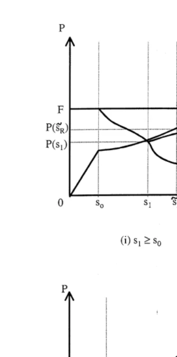
Proposition 1 is illustrated diagrammatically in Fig. 1. In each panel of Fig. 1 PC denotes the ‘participation constraint’, which is the locus of (s, P)-combinations such that (3) is satisfied. For any given s, we denote the corresponding P that exactly satisfies this constraint by P(s). Above (below) PC, P. ,s dp. Also using (2), (8) and (11), the slope of PC is:
an upward-sloping straight line: a higher private ownership share s raises p
proportionately, and P(s) rises correspondingly. For s.s , i*0 .0, and the
15
dependence of i* on s introduces curvature into PC. Iso-revenue loci are
illustrated in the figure by the dashed lines. These are found from (5), (8) and (11), and have slope:
Fig. 1. Revenue maximisation.
Higher loci represent more revenue. The loci are upward-sloping straight lines for
s#s , but curves for s0 .s .0
For any s, competition between potential buyers will always bid P up such that
the solution is on PC. Comparing (15) and (16), for s.s the slope of PC0 v the
slope of RR as sb1 /N. Hence in panel (i) there is a unique R-maximising
˜
solution, sR51 /N. In panel (ii) the highest RR-locus that can be reached is
˜
however, that in each panel P.0 in the solution: the government should not give
16
firms away and rely on its profit share for revenue.
We now modify Proposition 1 to allow for the more general welfare function
W(R, CS ). Note that, given the value of s, i* is determined, as consequently are R
and CS; the marginal rate of substitution W /W is therefore obtained.CS R
Proposition 2. When investment is in cost reduction, welfare W(R, CS ) is
˜ maximized by setting s5s :
W W
To explain Proposition 2 intuitively, suppose first that the government wishes to maximise CS. From (8), equilibrium output in each firm is increasing in i. Since i
is non-decreasing in s [Eq. (14)], but s#1, it follows that CS is maximized at
s51 (though this is only a unique solution if s0,1). In Proposition 2, however, we have the government valuing both R and CS, so that the optimum s is
˜
essentially a compromise between the R-maximising s (s5s from Proposition 1)R
˜
and the CS-maximising s (s51). The optimum value s5s is therefore in the
˜ ˜ ˜
range 1$s$s . Unlike in Proposition 1 part (i), the value of s in Proposition 2R
part (i) depends not just on N, but, through W /W , on all the parameters of theCS R
model. When part (i) of Proposition 2 applies, if the industry is a monopoly the government should transfer 100% of ownership to the private buyer, regardless of the specific form of W. For a duopoly, 50–100% should be transferred, the
˜
appropriate percentage depending on W /W . For NCS R 53, s[[1 / 3, 1], and so on.
˜
For any N, the precise solution for s depends on what welfare function is used. Suppose, for example, that W5R1CS, so that W /WCS R51, and that b51. From
If the government prefers revenue earlier rather than later, revenue via P is preferable to revenue via 12s. However, this does not necessarily lead to the conclusion that out of the multiple solutions
shown in panel (ii), s is the best. Once we take into account time preference for the government we0 should also take into account time preference for the potential buyers of the firm. This affects the price they are willing to pay and complicates the results considerably.
17
With W5R1CS, if s0.minh(21N ) / 2N,1jpart (ii) of Proposition 2 applies and the solution is
We note in Appendix A how Fig. 1 is easily amended to illustrate Proposition 2, with iso-welfare curves WW replacing iso-revenue curves RR. The tangency of an
WW curve with PC indicates the first-best value of s. However, if the weight on CS in the welfare function is relatively large, this tangency may occur at s.1, in
˜
which case the solution s51 is second-best.
Finally, notice that in some cases the optimum value of s does not depend on the cost function, so the government does not need ex ante information on this
function. This occurs with a general welfare function if N51, with a linear
welfare function W5R1CS if N51 or 2 and with either W5R or W5CS for
any N. Nonetheless, in all cases bidders need to know the cost function ex ante.
3.2. Investment in capacity expansion (CE)
We deal more briefly with Case CE (again with F unlimited) because the analysis is similar to that for Case CR. In Case CE unit costs at the production stage are fixed at c for all firms. Investment i is in capacity expansion, with output
always set at the capacity level: q5Q(i ). The investment and production stages
are, in effect, combined, yielding a Nash equilibrium i5i* in which i is chosen to
maximisep, subject to (10) and given the value of s. For an internal solution the f.o.c. is:
sQ9(i*) Af 2c2(N11)bQ(i*)g51 (17)
It is shown in Appendix A that A2c2(N11)bQ(i*).0 in this solution, and
also that for i*.0 it is necessary that s.s , where:0
s051 /Q9(0)(A2c) (18)
If s#s , then i*0 50 and so there is no output. This can happen as a result of a
combination of one or more of: a small ownership share s, a small markup A2c
and an investment function Q(i ) for which the first unit of investment has a relatively low productivity. From (17):
*
di
]
ds
2Q(i*) Af 2c2(N11)bQ(i*)g
]]]]]]]]]]]]]]] .2 0 for s.s0 5
5
s Qh 0(i*) Af 2c2(N11)bQ(i*)g2b(N11) Qf 9(i*)g j0 for s#s0
(19)
Proposition 3. When investment is in capacity expansion, revenue R is maximized
Part (i) of the proposition gives the internal solution that holds if s0,1. Here, if
˜
N51, sR51, the same result as found for Case CR. If N$2 an explicit solution
˜ ˜
for s is not obtained, but, as in Case CR, s is negatively related to N, and theR R
intuitive explanation is the same as that given for Proposition 1 part (i). Also, for
˜ ˜
s.s , ds / d(A0 R 2c).0 and ds / dbR ,0. A greater A2c and smaller b each
represent greater demand and so greater potential production profit P. The
government then optimally takes a greater share ofP.
Part (ii) of Proposition 3 describes what happens if s0$1. Here, whatever value
of s[(0,1] the government chooses, i is zero (as is P and q). There is no
privatisation in this case: the profit prospects of the industry are so poor that even
with s51, buyers who would invest in the industry cannot be found. It is still
possible to privatise the industry and have i.0, but this would require s to exceed
s , i.e. s0 .s0$1. In other words, a sufficiently large rate of subsidy forP would
18
enable privatisation to occur (with P.0); but we rule this out by assumption.
When we allow for CS in the welfare function we have the following parallel to Proposition 2.
Proposition 4. When investment is in capacity expansion, welfare W(R,CS ) is
˜ maximized by setting s5s :
WCS
Comparing this proposition with Proposition 3, note that, when there is
˜ ˜
privatisation, s$s . The intuition underlying this result is similar to that given forR
Proposition 2. For s.s , di* / ds0 .0, and so CS is increasing in s. When CS, as well as R, is valued by the government, there is therefore a rationale for raising s
18
˜
above sR (though it must also be taken into account that s cannot exceed 1).
Interestingly, if we take the illustrative welfare function W5R1CS, we find that ˜s51 for all N. The weight put on CS in this welfare function, and the associated
tendency to raise s to the maximum value, outweighs the tendency, if N$2, to
reduce s below 1 for revenue purposes. However, the urgency with which revenue is generally required in transition economies may make this particular welfare function unrealistic.
For the special case of b50, with unlimited international trade at price p5A,
˜ ˜
Propositions 3 and 4 yield sR5s51: regardless of the value of N and of whether
CS is included in the welfare function, the government should surrender all
ownership. With a constant output price there is no strategic interaction between firms, so that, in choosing s, the government can consider each firm separately. The argument for restricting s below 1 to limit revenue-damaging competition no longer applies.
Finally, note that, for Case CE in general, the government does not need to know the function Q(i ) if any of the following hold: N51, W5R1CS and b50.
Under any of these circumstances, it should set s51. Otherwise, however,
knowledge of Q(i ) is required by the government to set s appropriately.
3.3. Contractibility of investment
We now suppose, either for Case CR or Case CE, that the private owner’s investment is observable to the government and is therefore contractible. It therefore becomes feasible for the government to bear a share of (or to subsidise) investment costs. Given, however, that there is no limit on finance, the following proposition holds:
Proposition 5. Even if investment is contractible, to maximise revenue R the
government should not share in the cost of investment.
Note that the bearing of some of the cost of investment by the government cannot be ruled out on the grounds that it involves a direct cut in revenue R, for, ceteris paribus, it also results in the government receiving a higher price P for the firm. Rather, the rationale for this proposition is that, even without bearing any of the investment cost, the government is able to manipulate s to achieve a first-best solution. It is therefore unnecessary to use other policy instruments. In particular, suppose Eq. (2) is replaced by the more general equation:
p 5sP 2 si, 0,s #1 (29)
where s is an additional government policy tool, a parameter for the firm.
Proposition 5 implies that there is no advantage in making s other than unity.
government should not set s 5s. If it did so, we would havep 5ssP 2i , withd
the government taking a share s of overall profit p (rather than sharing only in
production profitP, as it does whens 51). In this case, maximisation ofpby the private owner yields a value of i* that is independent of s, so that the government loses all leverage over investment. As with any value ofs other than unity, R may
therefore be lower, and is never higher, than when s 51.
When consumer surplus CS is included in the welfare function a parallel to Proposition 5 does not hold unless the further restriction is made that s $1, i.e. unless subsidisation of investment is precluded. To see why this statement is true, note that in the analysis of Sections 3.1 and 3.2, if the weight the government puts
˜
on CS is sufficiently large, compared to that it puts on R, the solution s51 is not a first-best. A first-best could be achieved by setting s.1, but this is ruled out by
assumption. However, when investment is contractible, with Eq. (29) being used,
investment becomes a function of s /s, rather than just s. While retaining the
constraint that s#1, the possibility now arises of raising s /s above unity by
settings ,1, and thereby achieving the first-best solution. Thus, if we assume that subsidisation of investment (s ,1) is politically feasible, but subsidisation of
production profit (s.1) is not, it is desirable in this case that investment be
contractible. Alternatively, if the restriction s $1 is imposed, Proposition 5
generalises to the welfare function w5W(R, CS ).
4. Constrained finance
In the model of Sections 2 and 3 the new owner of a firm makes ‘up-front’
payments P1i, only receiving a return at the production stage. However,
transition economies suffer from severe imperfections in capital markets and sometimes from a general shortage of means of payment. It is therefore of interest to examine how the working of the model is affected if potential bidders for a firm have limited access to finance. To keep our analysis brief, we shall make the simplifying assumption that all potential bidders have the same amount of finance
19
F available. If bidders have formed coalitions, pooling their financial resources, this can be regarded as already reflected in the value of F.
The modifications that must be made to our previous analysis are illustrated in Fig. 2 for Case CR (we shall return to Case CE below). The first modification is that price P cannot exceed F. This is represented in the figure by the ‘finance constraint’ (FC):
19
Fig. 2. The effect of a shortage of finance.
FC: P5F (20)
Secondly, we introduce the ‘unconstrained investment boundary’ (UIB), which is given by:
UIB: P1i*(s)5F (21)
This is the locus of (s, P)-combinations for which, given any P, the investment
20
available. When s#s , i*(s)0 50 and so UIB reduces to P5F, i.e. UIB
coincides with FC. For s.s , however, it is found from (14) and (21) that UIB is0
downward-sloping. At (s,P)-combinations above UIB but below PC, the owner of the firm would like to set i5i*(s), but has only F2P,i*(s) available to spend.
In this case i5F2P. At (s, P)-combinations on or below UIB, i5i*(s).
The participation constraint PC from Fig. 1 is also shown, with the value of s at which it intersects UIB denoted by s . Panels (i) and (ii) in the figure show the1
cases of s1$s and s0 1,s , respectively. In panel (i) PC intersects the downward-0
sloping segment of UIB; in (ii) PC intersects the horizontal segment of UIB. In Section 3 PC was derived on the assumption that i5i*(s); but, now, for s.s , PC1
is above UIB and so investment i*(s) is infeasible. We therefore define a new ‘constrained participation constraint’, PC9. For s#s the finance constraint does1
not bind and so PC9coincides with PC; but for s.s , i1 5F2P,i*(s), causing
For any s, competitive bidding for firms will now lead to the attainment of a point
21
on whichever is the lower of PC9 and FC in the figure.
We can now generalize Proposition 1.
Proposition 6. When investment is in cost reduction and there is a limit on finance 9
F for each bidder, revenue R is maximized by setting s5s where:
R
If F is sufficiently large, there is no change from the solution described in
20
We assume for simplicity that in the production stage, when variable costs Cq are incurred, a firm pays its bills after sales revenue is received. The rationale for this assumption is as follows. First, the production stage may be regarded as implicitly representing an indefinitely repeated game, with a stream of payments into and out of the firm over time. Thus, out of the cost Cq incurred in the production stage, only a small proportion is payable before revenue is received. To treat this small proportion of Cq as pre-paid in the model would add complications without affecting results significantly. Second, insofar as there is trade credit or wage arrears, the pre-paid portion of Cq would be yet smaller.
21
In general, we cannot say whether, for s.s , PC1 9is above or below PC. This is because, for
Proposition 1. This solution appears as part (c) of Proposition 6. However, parts (a) and (b) of Proposition 6 relate to a value of F small enough to prevent Proposition 1 from applying, in which case the solution is definitely second-best. To illustrate these cases, panels (i) and (ii) of Fig. 2 replicate the corresponding panels of Fig. 1, with the limit on finance added. s , the level of s at which UIB intersects PC,1
now plays a critical role. Fig. 2(i) illustrates part (b) of Proposition 6. Here,
˜
although s exceeds s , it is less than s , the revenue-maximising value of s from1 0 R
Fig. 1(i). The solution depicted in Fig. 1(i) therefore cannot be achieved. Proposition 6 part (b) says that the government should set s5s in this case, so1
that P5P(s ). In effect, the solution here involves getting as close as possible to1
˜ ˜
s ,P(s ) , the solution in Fig. 1(i), while still remaining on PC. Intuitively, in Fig.
f
R Rg
˜
1(i), by setting s5s , the government obtains a particular combination ofR
immediate rewards (through P) and later rewards (through 12s). But the
introduction of the binding limit on a private owner’s ability to make up-front
payments, P1i, as in Fig. 2(i), causes the government to switch the emphasis
from its own immediate rewards to later ones, in the sense that it raises its ownership share 12s. Finally, part (a) of Proposition 6 is depicted in Fig. 2(ii).
As in part (ii) of Proposition 1, there are multiple solutions for s along PC9 5 PC, but the finance constraint imposes a limit F on the price P that can be paid. The range of multiple solutions is therefore more restricted than in Proposition 1.
It is now a simple matter to allow for CS in the welfare function.
Proposition 7. When investment is in cost reduction and there is a limit on finance
F for each bidder, welfare W(R, CS ) is maximized by setting:
˜
9
(a) s5s if sR 1#s or s0 R.s1.s ;0
˜
(b) s5s otherwise.
This proposition states that if there is a binding limit on finance then the
9
solution s5s , which maximises R, also maximises W(R, CS ); otherwise, F doesR
not affect the solution, which is therefore given by Proposition 2. Take, for example, the situation depicted in Fig. 2(i). We already know that R-maximisation is achieved by setting s5s , but consider how CS is affected by variation of s.1
First, for s#s , the limit on finance does not bind and so i and CS are increasing1
in s. Second, for s$s , if s is raised, then, ceteris paribus, the firm is more1
profitable to a buyer. Its price P is therefore bid up (there is rightward movement
22
along PC9, which is upward sloping). However, because finance is limited, this
leaves the new owner with less to spend on investment, so that CS is reduced. It follows that CS, as well as R, is maximized at s5s .1
We can also consider the effect of the limit on finance in Case CE.
22
Proposition 8. When investment is in capacity expansion Propositions 6 and 7
still hold except that, if s #s , the industry is not privatised.
1 0
In Case CE Fig. 2 again applies except that the straight-line section of PC must be deleted in each panel. This has a significant effect on the solution in panel (ii),
in which case privatisation does not occur. For s#s there are no bidders for0
firms. For s.s competitive bidding pushes P towards F, but as P approaches F0
the new owner of a firm has no finance left to invest in capacity and so a firm is not worth buying, i.e. an equilibrium value of P does not exist. Setting b50, so that there is unlimited international trade at price P, does not affect the validity of Proposition 8.
Broadly speaking, we have therefore found in this section, for both cases, CR and CE, that a binding limit on finance tends to reduce the share of ownership that the government should keep. Suppose, for example, that an industry is sold off to foreign buyers, perhaps because it requires particular reorganisational skills that are not available domestically. If the foreign buyers have a relatively large amount of finance available, then the state ownership share in this industry should be kept relatively low. However, we are disregarding here the political tensions that may
23
accompany extensive foreign ownership.
5. Further discussion
We have shown that market structure has a significant role to play in the choice of an appropriate privatisation policy. A limitation of our paper, however, is that we have not allowed for uncertainty. Demougin and Sinn emphasise the risk-sharing benefits of state participation in the ownership of privatised firms. By excluding this factor we presumably bias our results against state ownership. Also, we make no allowance for the regulatory regime that might be operated after
24
privatisation. We end the paper by discussing the extent to which our results are
dependent on some of our other assumptions.
23
Also, note that once the constraint on finance is introduced, the argument made in Section 3.3 about the irrelevance of contractibility under some circumstances does not apply. Even ifs 5s in Eq.
(29), so thatp 5ssP 2i , the government now has some leverage over investment: a rise in s isd
associated with a higher P, and so reduces the funds F2P that the owner has available for investment.
24
First, we might introduce the assumption that the government could restrict the price at which firms are sold below the competitive level. With unconstrained finance this would be of no benefit, for nothing that happens after the sales stage is affected by the level of P. When finance is constrained, however, restriction of P, for any given s, can increase investment. In fact, as we show in Appendix A, if the government wishes to maximise revenue it should never restrict P in this way. If, however, it wishes to maximise CS (i.e. to maximise i ) the solution may be to set
P50. In terms of Fig. 2, the government wants both to raise s as far as possible
¯
and, for any s, to restrict P such that i is unconstrained. If UIB cuts the s axis at s,
¯ ¯
the government should therefore set s5minh1, sj, and if s5s is the solution here,
P50. This conclusion holds for both Case CR and Case CE and is the one
situation in our analysis in which the government should give the firm away. Secondly, we might assume that instead of selling a share in the ownership of firms, the government gives it away to the general population (voucher privatisa-tion). Thus, the government obtains revenue only from selling the remaining share of firms, not from continued ownership. With dispersed ownership, we may assume that the general population does not try and influence firm behaviour. Our analysis could then be reworked, perhaps with Eq. (29) rather then Eq. (2), with three arguments in the welfare function-revenue for the population as a whole, revenue for the government and consumer surplus.
A third modification would be to allow for competition from imports or de novo firms. However, at least on one interpretation, such competition can be treated as being implicitly taken into account already. We may think of our model as being part of a larger model in which goods are differentiated. Suppose that our privatised firms produce goods with one set of characteristics, while imports and the output of de novo firms have other characteristics (see Bennett et al., 1999). Consider a simple differentiated-good model in which the demand for each type of good depends linearly on the set of prices. Given the prices fixed by importers and de novo firms, our analysis would still hold. If importers or de novo firms reduced their price, however, there would be a vertical fall in the demand curve for the output of the privatised firms. In other words, it would simply cause a reduction in
A in Eq. (1). Among the consequences would be that s0 would rise and so a solution with zero investment in Case CR and no privatisation in Case CE would be more likely to hold.
Acknowledgements
We are grateful for very helpful comments by the editor, Thomas Piketty, an anonymous referee, Istvan Abel, Stanislaw Gomulka, Ian MacIntyre, Stephen Salant, Andrew Weiss and seminar participants at Bath, Heriot-Watt, Leicester and Oxford Universities, and at the London School of Economics and the CEPR / WDI International Workshop in Transition Economies, Prague, July 1998. The usual disclaimer applies.
Appendix A
Existence and uniqueness of investment: Case CR: Using (11), define the function G(i ) as:
solution must exist if G(0).0, the condition for which is:
2 2b(N11)
¯ ]]]]
A2C C9(0).
f
g
2NsThe definition of s0 follows from this condition. To establish uniqueness, it is
sufficient to show that G9(i ),0 for all s.s , i.e.:0
Proof of Proposition 1. (i) Along PC all profitp is bid away. Using (2), (3) and
2
(8) to substitute into (5) gives R5NshfA2C(i*) /(Ng 11) /bj 2i* . Differentiat-d
1
]
ing with respect to s and using (11) yields the f.o.c., N(di* / ds)
h
Ns21j
50. Concavity of W ensures that the s.o.c. is satisfied. The corner solution, s51, can˜
1) , so that the government is indifferent between all points in (0,minhs ,10 j]. Because s0$1 /N, any s.s must imply a lower level of revenue (from part (i) of0
the proof), so the result follows.
Proof of Proposition 2. (i) Differentiating (4) and using (2), (3), (5), (6), (8) and
the solution follows. The s.o.c. is satisfied, given that W(?) is concave. (ii) Totally
2
¯
differentiating (4) when i50 gives dP/ ds5
fs
A2C /b(Nd
11) . The proof theng
follows as for Proposition 1 part (ii). By assumption, s#1.The iso-R curves of Fig. 1 must be replaced with iso-W curves. From (4), (8), (9) and (11) an iso-W curve has slope:
2 W
dP 1 A2C(i*) 1 CS di*
] ] ]]]
F
G
]] ]] ]WW: 5 2
F
2(12s)1NG
(A.1)ds b sN11d 2Ns WR ds
˜
Suppose first that a positive-i* solution holds (s.s ). Equating the slopes of PC0
and WW we obtain the value of s shown in part (i) of the proposition. If this value of s exceeds unity, we have a corner solution s51. Apart from this qualification, panel (i) of Fig. 1 applies in this case, but with the RR-loci relabelled WW and
1
]
1 /N relabelled 1 /N12W /W . With similar relabelling, panel (ii) of Fig. 1CS R
depicts part (ii) of Proposition 2. This case occurs if, at (s ,P(s )), the slope of the0 0
curved segment of PC is less than the slope of the curved segment of WW. Then,
i*50 in the solution.
Existence and uniqueness of investment: Case CE: Using the f.o.c. (17), define the function H(i ) as:
H(i )5sQ9(i*) Af 2c2(N11)bQ(i*)g21
As i→`, H(i )→21. Function H(i ) is continuously defined for all i$0, so if
H(0).0 a solution must exist. The definition of s follows directly from this.0
Differentiating H(i ) w.r.t to i at i*:
2
H9(i*)5s Qh 0(i*) Af 2c2(N11)bQ(i*)g2(N11)b Qs 9(i*)d j Substituting from (17) gives H9(i*),0 and so the solution is unique.
To show that A2c2(N11)bQ(i*).0, note that with production taking place,
there is a positive cost to investment. This implies that marginal revenue must be
greater than the marginal unit cost c, or A22bNQ(i*)$c, from which the proof
follows.
Proof of Proposition 3. Along PC all profitp is bid away. Using (2), (3) and (10) to substitute into (5), R5sA2bNQ(i*)2c Q(i*)d 2i*. Differentiating with
re-spect to s gives the f.o.c. hsA22bNQ(i*)2c Qd 9(i*)21 (di* / ds)j 50. Using (17)
to substitute for Q9(i*) then gives the internal solution of part (i) of the
proposition. The s.o.c. is satisfied because W is concave. From the f.o.c., at s5s0
a rise in s reduces (increases) R if (A2c)Q9(0)21,(.)0, i.e. using (18), as
s0.(,)1. If s0$1 i50 for all s[(0,1]. Part (ii) of the proposition follows.
Proof of Proposition 4. Differentiating (4) w.r.t. s and using (2), (3), (5), (6) and
di* 2
]ds
h
fQ9(i*) As 2c22bNQ(i*)d21 Wg R1f
bN Q(i*)Q9(i*) Wg j
CS 50Substituting from (17) and rearranging, part (i) of the proposition is obtained. Concavity of W guarantees that the s.o.c. is satisfied. Part (ii) follows as for Proposition 3.
Proof of Proposition 6. (a) If s#s , i*0 50. RR and PC curves are parallel (as shown w.r.t. Proposition 1), so R is constant along PC. From Proposition 1, if
s1#s , R is lower for all s0 .s than for s0 #s . Therefore, the government is0 9
indifferent to any sR[(0,minhs , 11 j]. (b) Consider first s[[s , 1]. In this interval,1
competitive bidding ensures the firm is on the lower of FC and PC9. Along FC,
F5P, so that i50 and therefore, from (8), P is independent of s and P. From (5), it follows that dR / ds,0. s should therefore be reduced at least to the level at
which PC9 intersects FC. Hence, the solution lies along PC9 below FC.
2
Using i5F2P, (2), (3) and (8), along PC9, s Af 2C(F2P) /b(Ng 11) 2F5
0. Substituting from this equation for s in (5) and also using i5F2P and (8), R
is expressed as a function of P, from which:
dR 2 Af 2C(F2P) Cg 9(F2P)
]dP511]]]]]]]]2
b(N11)
Note that if the constraint F is just loose enough to enable the firm to choose its
optimal unconstrained i (i.e. F5P1i*(s)) we have from (11) that if s51 /N,
2
A2C(F2P) C9(F2P)5 2b(N11) / 2. Since, for s.s , when the constraint
f g 0
bites (i.e. F,P1i*(s)) i,i*(1 /N ) and also from (12), d Ahf 2C(F2P) Cg 9(F2 2
P) / dij .0, it follows that A2C(F2P)C9(F2P), 2b(N11) / 2. Hence dR / dP,0, so that on s[fs ,1 , R is maximized at s1 g 5s . From Proposition 1, on1
s[(0,s ], R is maximized at s1 5s . s is therefore the optimum value of s.1 1
Proof of Proposition 7. (a) From the proof of Proposition 5, for s.s dR / dP1 ,0,
2 2
and from (6) and (8) dCS / dP5N Af 2C(F2P) Cg 9(F2P) /b(N11) ,0.
˜
Therefore, from (2), dw / dP,0. So if sR.s , welfare is maximized on s1 [[s ,1]1
˜ ˜ ˜ ˜
at s5s . From Proposition 2, s1 $s ; so if sR R.s , s1 .s . In the absence of a1
˜
limit F, dW/ ds.0 for s[[s ,s ]. But when there is a limit F it has no effect for0
s#s . Hence, W is maximized on s1 [[s ,s ] at s0 1 5s . (b) This follows from1
Proposition 4.
Proof of Proposition 8. First consider Proposition 5. Investment is decreasing in s
dP Q(F2P) Af 2c2bNQ(F2P)g
]
U
p 505]]]]]]]]]].0ds sQ9(F2P) Af 2c22bNQ(F2P)g
˜
For s.s , i1 5F2P. Along PC9, dP/ ds.0, so di / ds,0. If s.s , s1 1 must therefore maximise R over s[[s ,1]. For s1 [(s ,s ], dR / ds0 1 .0 (from Proposition 3). s5s is therefore the optimum s.1
Turning to Proposition 6, from the first part of this proof, for s.s , dR / ds1 ,0.
2
Differentiating (6) w.r.t. P gives dCS / dP5 2bN Q(F2P)Q9(F2P),0. The
proof is then the same as for Proposition 6.
Effect on R of Restricting P: For s,s the firm’s behaviour is not constrained1
by a shortage of finance. Any restriction of P below the competitive level reduces
R. Suppose that s$s . In Fig. 2(i) define loci PC1 9 2k, where k is a non-negative
constant. It was shown in the proof of Proposition 5 that, for s$s , R is greater as1
we move to the left on PC9. Along any locus PC9 2k the same property applies, so R is greatest at the intersection of the locus with UIB. We have shown in
Proposition 5 that along UIB for s$s , R is maximized at s1 5s . But at s1 5s ,1
the firm is on PC9, so there is no restriction of P. This applies for both Case CR and Case CE
References
Bennett, J., Estrin, S., Hare, P., 1999. in press. Output and exports in transition economies: A labor management model. Journal of Comparative Economics 27, 295–317.
Blanchard, O.J., 1994. Transition in Poland. Economic Journal 104, 1169–1177.
Bolton, P., Roland, G., 1992. Privatisation in Central and Eastern Europe. Economic Policy 15, 276–309.
Brada, J.C., 1996. Privatisation in Central and Eastern Europe. Journal of Economic Perspectives 10(2) (Spring), 67–86.
Coricelli, F., 1996. Fiscal constraints, reform strategies and the speed of transition: The case of Central–Eastern Europe, CEPR Discussion Paper No. 1339.
Demougin, D., Sinn, H.-W., 1994. Privatisation, risk taking and the Communist firm. Journal of Public Economics 55, 203–231.
Dewatripont, M., Roland, G., 1996. Transition as a process of large-scale institutional change. Economics of Transition 4, 1–30.
Duponcel, M., 1998. Restructuring food industries in five Central and Eastern European front-runners towards EU membership, Discussion Paper No. CERT 98 / 6, Heriot-Watt University.
EBRD, 1995. Transition Report 1995, EBRD, London.
EBRD, 1996a. Transition Report Update, April 1996, EBRD, London. EBRD, 1996b. Transition Report 1996, EBRD, London.
EBRD, 1997. Transition Report Update, April 1997, EBRD, London.
Estrin, S. (Ed.), 1994. Privatisation in Central and Eastern Europe. Longman, London, New York. Fershtman, C., Judd, K., 1987. Equilibrium incentives in oligopoly. American Economic Review 77,
927–940.
Gaddy, C., Ickes, B., 1998. Underneath the formal economy: Why are Russian enterprises not restructuring? Transition (August).
Linz, S., Krueger, G., 1998. Enterprise restructuring in Russia’s transition economy: Formal and informal mechanisms. Comparative Economic Studies 40, 5–52.
Perotti, E., 1995. Credible privatisation. American Economic Review 85, 847–859.
Salant, S.W., Shaffer, G., 1999. Unequal treatment of identical agents in Cournot equilibrium. American Economic Review 89, 585–604.
Sinn, G., Sinn, H.-W., 1993. Jumpstart. MIT Press, Cambridge, MA.
Sinn, H.-W., Weichenrieder, A., 1997. Foreign direct investment, political resentment and the privatisation process in Eastern Europe, Economic Policy (April), 179–209.