International Review of Economics and Finance 9 (2000) 209–222
Adjusting for risk:
An improved Sharpe ratio
Kevin Dowd*
University of Nottingham Business School, Jubilee Campus, Nottingham, NG8 1BB, UK Received 4 March 1999; accepted 19 July 1999
Abstract
This paper proposes a new rule for risk adjustment and performance evaluation. This rule is a generalization of the well-known Sharpe ratio criterion, and under normal conditions enables a manager to correctly assess alternative risky investments. The rule is superior to existing rules such as the standard Sharpe rule and the RAROC, and can make a substantial difference in estimates of required returns. 2000 Elsevier Science Inc. All rights reserved.
JEL classification:G10; G11
Keywords:Sharpe ratio; Risk adjustment; Performance evaluation
1. Introduction
As is well known, the general problem of risk adjustment has two main aspects. The first is adjustment before the event, the typical case being that of investment managers choosing between alternative risky investment opportunities. How do they choose between investmentA, which has a high expected return and a relatively high risk, and investment B, which has a low expected return but is relatively safe? We can answer this question only if we have some means of adjusting expected returns for risk. We therefore have to adjustexpectedreturnsbeforewe take on the relevant risk. The second side of the problem is that of evaluatingactualinvestment performance
after the event, when decisions have already been made and the results of those
decisions are apparent. For example, we may need to compare traderA, who made a high profit but took a lot of risks, with trader B, who made a low profit but took
* Corresponding author. Tel.:144-115-846-6666; fax:144-115-846-6667. E-mail address:[email protected] (K. Dowd)
210 K. Dowd / International Review of Economics and Finance 9 (2000) 209–222
few risks. To distinguish between these two aspects of risk adjustment, we normally use the term “risk adjustment” to refer to the first, ex ante, aspect, and we usually refer to the second, ex post, aspect as “performance evaluation.”
This paper derives an operational decision rule that will enable a manager to correctly assess alternative investment opportunities or past investment decisions, where the alternatives usually have differing (expected or realized) returns and risks. Section 2 sets out the uses of risk adjustment and performance evaluation measures. Section 3 assesses the traditional or standard Sharpe ratio approach. If returns are normal, the standard Sharpe ratio gives the correct result if the investments being considered are independent of the rest of our portfolio, but cannot be relied upon otherwise. Section 4 then sets out the generalized Sharpe ratio that is free of this latter limitation and is valid regardless of the correlations of prospective investments with our portfolio. This section also gives some numerical examples to illustrate that the generalized and traditional Sharpe rules can lead to very substantial differences in estimates of required returns, and so lead to very different assessments of prospective or past investment decisions. It goes on to show how the rule can also be expressed using value at risk (VaR) rather than the standard deviation of returns as our risk measure. It also develops the generalized Sharpe rule for both the simple case of a cash benchmark asset, and for the more general case of a risky benchmark asset; and presents some further numerical examples that suggest that the treatment of the benchmark asset can make a considerable difference in estimates of required returns. Overall, these results suggest that the generalized Sharpe rule is a distinct improvement on the traditional Sharpe rule, but also indicate that considerable care needs to be taken over the benchmark.
2. The need for risk adjustment and performance evaluation
Measures of risk adjustment and performance evaluation have a number of impor-tant uses. The first is the obvious one of enabling us to compare the returns associated with different levels of risk, either those returns expected ex ante or those actually made ex post. Risk adjustment gives us a metric that enables us to choose between investment opportunities with differing (expected) returns and risks. Similarly, perfor-mance evaluation gives us a metric that enables us to compare the perforperfor-mance of units or portfolios that made different returns but also took different risks.
to position limits that are determined on the basis of its risk-adjusted profitability relative to other business units in the organization.
Performance evaluation measures are also important in framing appropriate com-pensation rules. If management wishes to maximize risk-adjusted profits, as they should be, it is essential that it use compensation rules based on risk-adjusted rather than raw profits. If management rewards traders or asset managers on the basis of actual profits, traders (and asset managers) will seek to maximize profits to boost their bonuses, and they will do so with insufficient concern for the risks they are taking.1 Those who read the financial press will need no reminding of this problem.
It makes no sense for management to reward traders for taking excessive risks and
then worry about how to control their excessive risk-taking. Instead, management should manage their risk-taking in the context of incentive structures thatencourage
their traders to take the levels of risk that management wants them to take. If manage-ment wishes to encourage traders to take account of the risks they inflict on the institution, it should reward them according to risk-adjusted (rather than raw) profits. Traders will then maximize risk-adjusted profits, and the conflict of interest that would otherwise exist between the institution and its traders will be significantly ameliorated.
3. The traditional Sharpe ratio approach2
But how do we carry out the risk adjustment? The traditional approach is to use a Sharpe ratio. Suppose we have a portfolio,p, with a return Rp. We also observe a benchmark portfolio, denoted by b, with return Rb. Let d be the differential return
Rp 2 Rb, and let de be the expected differential return. We can now define the ex ante Sharpe ratio by Eq. (1):
SRante 5de/se
d, (1)
where se
d is the predicted standard deviation of d. This ratio captures the expected differential return per unit of risk associated with the differential return, and takes account of both the expected differential return between two portfolios and the associated differential risk. Since it gives risk estimates before decisions are actually taken, the ex ante Sharpe ratio can be very useful for decision-making (e.g., choosing investments).
We can also define the ex post Sharpe ratio by Eq. (2):
SRpost 5d/s
d, (2)
wheresdis the standard deviation ofdover a sample period. This version of the ratio
takes account of both the ex post differential return and the associated variability of that return, and can be very useful for performance evaluation after the event.
212 K. Dowd / International Review of Economics and Finance 9 (2000) 209–222
is bad. When choosing between two alternatives, the Sharpe ratio criterion is therefore to choose the one with the higher Sharpe ratio. If we are deciding on investments before the event, we would choose that investment with the highest ex ante Sharpe ratio; if we are trying to evaluate traders after the event, we would give higher marks to the trader with the higher ex post Sharpe ratio.
It is important to appreciate that the Sharpe ratio always refers to thedifferential
between two portfolios.3We can think of this differential as reflecting a self-financing
investment portfolio, with the first component representing the acquired asset and the second reflecting the short position—in cash or in some other asset—taken to finance that acquisition. As Sharpe explains,
Central to the usefulness of the Sharpe ratio is the fact that a differential return represents the result of a zero-investment strategy. This can be defined as any strategy that involves a zero outlay of money in the present and returns either a positive, negative, or zero amount in the future, depending on circumstances. A differential return clearly falls in this class, because it can be obtained by taking a long position in one asset (the fund) and a short position in another (the benchmark), with the funds from the latter used to finance the purchase of the former. [Sharpe (1994, p. 52)]4
The Sharpe ratio gives us sufficient information to choose between two investment options ex ante or evaluate the better of two trading units ex post,providedthe returns to the two assets in question (or the two traders’ portfolios) are uncorrelated with the returns to the rest of the institution’s portfolio.
If we are choosing between alternatives, we pick the alternative with the higher Sharpe ratio; if we are ranking investments, we rank the investment with the higher Sharpe ratio ahead of the investment with the lower one.5 Nonetheless, if we can
compare investments on a bilateral basis, we can also compare investments within a larger group as well, subject to the qualifier about zero correlation with the portfolio. If investment A has a higher Sharpe ratio than investment B, and B has a higher Sharpe ratio thanC, and so on, we rank investmentAfirst, followed byB,C, and so on. The relevant bilateral comparisons between different investments enable us to rank all our investments on a risk-adjusted basis. The higher the Sharpe ratio, the higher the risk-adjusted return. In effect, we can take the Sharpe ratio to be a proxy for the risk-adjusted return.6
the rest of our portfolio mean that the Sharpe ratio criterion cannot generally be relied upon to give the right answer.7
4. A generalized Sharpe approach
4.1. The generalized Sharpe ratio
Fortunately, this problem with the traditional Sharpe ratio is easily put right. Sup-pose we have a current portfolio and are considering buying an additional asset. To get around this correlation problem, all we need to do is construct two Sharpe ratios, one for the old (or current) portfolio taken as a whole, and one for the new portfolio (or the portfolio we would have if the proposed trade went ahead), also taken as a whole. If we denote the old Sharpe ratio by SRold, and the new one by SRnew, the decision rule is very simple, as shown in Rule/Eq. (3):
Buy the new asset (i.e., go from old to new) if SRnew >SRold. (3)
We go for the new portfolio if it has a Sharpe ratio greater than or equal to that of the old portfolio. The optimality of this rule follows from the previous discussion, which told us that we should choose the position with the highest Sharpe ratio if two positions are uncorrelated with the rest of our portfolio—and this condition is now automatically satisfied.8
This generalized Sharpe rule avoids the correlation problem we encountered with standard applications of the Sharpe ratio. The correlation of any new position to the old portfolio can take any value, not just zero, and its value is already implicitly allowed for in the denominator ofSRnew.This rule is therefore valid for any correlations
of the prospective new asset with our existing portfolio, unlike traditional applications of the Sharpe ratio that are valid only if the correlation is zero.
It remains to spell out the details. Suppose we are deciding whether to make an investment decision involving the purchase of a new assetAwith a short position in the benchmarkb, and we assume for simplicity that the benchmark asset is cash. This latter assumption implies that the benchmark return, Rb, is zero. (I shall relax the assumption of a cash benchmark in due course.) I shall also drop the expectation superscripts to keep the notation from becoming too cumbersome. The differential return,dold, is thereforeRold
p , and the standard deviation is sdoldp , or soldRp. The ratio of Rold
p tosoldRpthen gives us our existing (old) Sharpe ratio. Now suppose that the
prospec-tive new portfolio consists of the new asset Aand the existing portfolio, in relative proportionsa and 1-a. The expected return on the new portfolio is therefore shown by Eq. (4):
Rnew
p 5aRA1 (12a)Roldp (4)
Given thatRb is zero, (4) is equal to the expected differential for the new portfolio,
dnew. Similarly, the assumption of a cash benchmark also enables us to say that snew d equal to snew
Rp. Using (3), we should therefore make the investment if, as shown in
214 K. Dowd / International Review of Economics and Finance 9 (2000) 209–222
SRnew 5dnew/snew
Rp > dold/soldRp 5SRold (5)
Substituting into Eq. (5) and rearranging, our criterion becomes Eq. (6):
RA >Roldp 1[snewRp /soldRp 21]Roldp /a (6)
Eq. (6) tells us that the expected return on assetAmust be greater than or equal to the expression on the right-hand side if the asset is to be worth acquiring. The expression on the right-hand side of (6) can therefore be interpreted as the required return on assetA.This required return consists of the expected return on the existing portfolio plus an adjustment factor or risk premium that depends on the risks in-volved—and, more specifically, rises with the ratio of new to old portfolio standard deviations. Eq. (6) tells us, as we would have expected, that the more the new asset contributes to overall portfolio risk, the greater the expected return required to make its acquisition worthwhile. There are also some other implications:
• The new asset’s risk is only relevant to the decision whether to acquire the new asset insofar as it affects overall portfolio risk: the volatility of the new asset’s return does not enter the decision rule other than through the portfolio risk snew
Rp. This reflects the well-known result in portfolio theory that the risk that matters is not an asset’s own individual volatility, but its contribution to the risk of the portfolio as a whole.
• In the special case where the new asset adds nothing to overall portfolio risk (i.e., wheresnew
Rp is equal tosoldRp), the right-hand side of (6) boils down toRoldp and the decision rule merely requires the new asset have a net return at least as great as that from the existing portfolio.
• If the new asset increases overall portfolio risk (i.e., ifsnew
Rp is greater thansoldRp), we should expect the new asset to earn a return greater than Rold
p to be worth acquiring. We need the greater return as compensation for the greater portfolio risk its purchase would involve. Conversely, if the asset makes a negative contribu-tion to portfolio risk, its required return is less than that of our existing portfolio.
4.2. Some illustrative examples
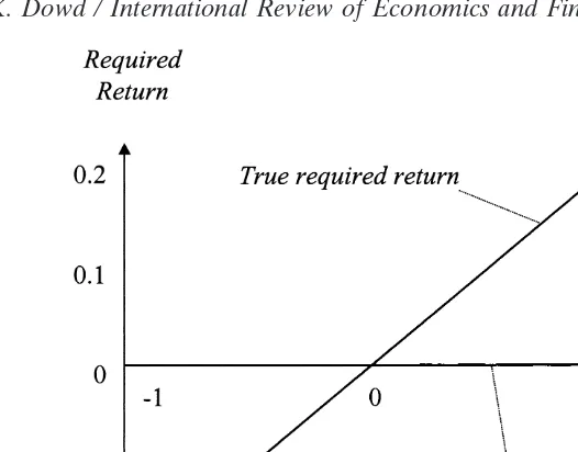
Some illustrative required returns are given in Fig. 1. The upward-sloping line gives the required returns generated by the generalized Sharpe rule for various possible correlations between a prospective asset acquisition and our existing portfolio, for a given plausible set of parameter values.9 The higher the correlation, the more the
Fig. 1. Required returns: generalized vs. traditional Sharpe ratio.
Fig. 1 also illustrates how the traditional Sharpe rule can give misleading answers to decision-making problems. Since it ignores the true correlation between any pro-spective new position and our existing portfolio, it is effectively the same as our generalized Sharpe rule with the correlation arbitrarily assumed to be zero. It will therefore imply a required return that is independent of the correlation (i.e., is hori-zontal, in terms of Fig. 1) and give unbiased answers if and only if the true correlation also happens to be zero. This is reflected in Fig. 1 where the two required returns cross at the zero-correlation point. However, the traditional Sharpe rule will give biased answers wherever the true correlation is not zero:
• If the correlation is positive, the traditional Sharpe rule will underestimate the true required return, and therefore lead to incorrect asset acquisitions. For example, if the true correlation is 0.5, the traditional Sharpe rule will lead us to accept any assets with more than negligible expected returns, whereas the “true,” generalized, Sharpe rule says that we should only accept new acquisitions with expected returns of at least 10%. The use of the traditional Sharpe ratio in this case will therefore lead to incorrect acquisitions whenever the expected return is positive but less than 10%.
• If the correlation is negative, the traditional Sharpe rule overestimates the re-quired return, and leads to incorrect decisionsnot to acquire new assets. Thus, if the correlation is20.5, the true required return is minus 10%, but the traditional Sharpe rule mistakenly estimates it to be (about) zero. We will then reject all new positions with negative expected returns, even though such positions would be good for us provided the expected return is more than minus 10%.
decision-216 K. Dowd / International Review of Economics and Finance 9 (2000) 209–222
Fig. 2. Required return and the VaR elasticity.
making where the true correlation is nonzero. It will lead us to mistakenly acquire new positions if the correlation is positive, and to mistakenly reject new positions if the correlation is negative. The distortion in decision-making also gets bigger, the further away the correlation is from zero.
4.3. The generalized Sharpe rule in VaR form
We can also write Eq. (6) in an equivalent form, using VaR instead of portfolio standard deviation as our risk measure. Assuming normality, we can infer Eq. (7):
snew
Rp/soldRp 5VaRnew/VaRold (7)
where VaRnew is the VaR of the new portfolio and VaRold is the VaR of the old portfolio.10We now rearrange these expressions to put the standard deviations on the
left-hand side and use the rearranged expressions to substitute out the standard deviations from Eq. (6). Our decision rule (6) then becomes Eq. (8):
RA >Roldp 1(VaRnew/VaRold21)Roldp /a (8)
Noting that the incremental VaR,DVaR, is equal toVaRnew2VaRold, and rearranging, Eq. (8) becomes Eq. (9):
RA >Roldp 1(DVaR/VaRold)Roldp /a 5[11 hA(VaR)]Roldp (9)
where hA(VaR) is the percentage increase in VaR occasioned by the acquisition of the position in asset A divided by the relative size of the new position. hA(VaR) is therefore the elasticity of our VaR with respect to the new asset position.
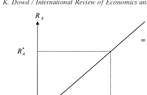
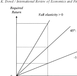
Fig. 3. Required returns and VaR elasticities.
horizontal axis to the vertical axis via a diagonal line with a slope of one plus the VaR elasticity. If the expected portfolio return is Rold*
p , the required return will be
R*A. Any asset with an expected return greater than or equal toR*A will then be worth acquiring, and any asset with a lower expected return will not be.
The higher the VaR elasticity, the higher the required return, for any given value ofRold
p . Some illustrative examples are shown in Fig. 3. If the VaR elasticity is positive, the new acquisition would add to overall risk and have a required return greater than
Rold
p . We require the higher return to compensate for the higher risk. If the VaR elasticity is negative, on the other hand, the new acquisition would reduce overall risk and have a required return less than Rold
p . We would be prepared to accept a lower expected return because the new acquisition would reduce our risks. It is also possible for the VaR elasticity to be less than minus 1. In this case, one plus the VaR elasticity would be less than zero and the required return would be negative. This is of course another illustration that people will sometimes pay (i.e., bear a negative return) for a hedge position.
4.4. The generalized Sharpe ratio with a noncash benchmark
218 K. Dowd / International Review of Economics and Finance 9 (2000) 209–222
of the differential, sd, will then no longer be equal to sRp, but instead be given by Eq. (10):
sd5
√
s2Rp 1 s2Rb 22rRp,RbsRpsRb (10)where the “old” and “new” superscripts are dropped for convenience. The analysis runs parallel to the earlier derivations, but this time our decision rule [i.e., the analog of (6), or (9), in VaR form] is to acquire the new position if, as shown in Eq. (11):
RA 2Rb >(Roldp 2Rb) 1(snewd /soldd 21)(Roldp 2 Rb)/a (11)
Sinced is the difference between the relevant (i.e., old or new) portfolio return and the benchmark return, we can regard the standard deviation of d as the standard deviation of the return to a combined position that is long the relevant portfolio and short the benchmark. This combined position has its own VaR, which Dembo (1997, p. 3) calls the benchmark-VaR, or BVaR.11Assuming normality, the ratio of standard
deviations in (11) is then equal to the ratio of new to old BVaRs, as given by Eq. (12):
snew
d /soldd 5BVaRnew/BVaRold (12)
We now substitute (12) into (11) and rearrange to write (11) in its BVaR form, as shown in Eq. (13):
RA 2Rb >[11hA(BVaR)](Roldp 2Rb) (13)
This rule is an exact analog of our earlier rule [i.e., (9)], but withRA 2Rband Roldp 2
Rbinstead ofRAandRoldp , and the BVaR elasticity instead of the earlier VaR elasticity. Incidentally, (13) also tells us that the relevant risk measure (and, hence, the term that enters into the risk premium in the required return condition) is the BVaR elasticity rather than the VaR elasticity. Put differently, the VaR elasticity is the correct elasticity to useonlyin the special case where the benchmark is cash, in which case the BVaR collapses to the VaR and the two elasticities are the same.
This decision rule can be represented by a figure analogous to our earlier Figure 2. Fig. 4 is the same as Fig. 2, except that we have now have the differentials between the relevant returns and the benchmark return, and the elasticity is in terms of BVaR rather than VaR.
We might also wonder what error we are likely to make if we incorrectly assume that the benchmark is cash and hence incorrectly takeRbandsRpto be zero. To address this question we first rewrite Eq. (13) as Eq. (14):
RA >[11 hA(VaR)]Rpold1[hA(BVaR) 2 hA(VaR)]Roldp 2 hA(BVaR)Rb (14)
Comparing the right-hand sides of (9) and (14) then gives us Eq. (15):
‘True’ required return5Required return with assumed cash benchmark
1[hA(BVaR) 2 hA(VaR)]Rold
p 2 hA(BVaR)Rb (15)
If we mistakenly use a cash benchmark, we would therefore estimate the required return with an error of [hA(BVaR) 2 hA(VaR)]Rold
Fig. 4. Required returns with a noncash benchmark.
depends onRold
p ,Rb, and both the BVaR and VaR elasticities. The error will generally be nonzero, and be zero only in the special cases where the elasticities both happen to be zero, or whereRold
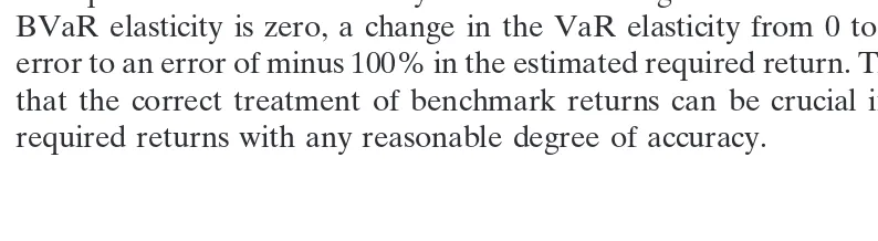
p just happens to be equal tohA(BVaR)Rb/[hA(BVaR)2 hA(VaR)]. Some illustrative numbers are given in Table 1 for various assumed elasticity values, on the hypothetical assumption that we are dealing with an portfolio return of 0.2 and a benchmark return of 0.1. These results indicate that the inappropriate use of a cash benchmark can easily produce very large errors in the estimation of required return. Errors are frequently plus or minus 100% of the true required return, and the signs of the errors depend on both elasticities. These results also indicate that errors in estimates of required returns can be very sensitive to changes in elasticities. For example, if the BVaR elasticity is zero, a change in the VaR elasticity from 0 to 1 leads from a zero error to an error of minus 100% in the estimated required return. These results illustrate that the correct treatment of benchmark returns can be crucial if we are to estimate required returns with any reasonable degree of accuracy.
Table 1
Illustrative errors from the inappropriate use of a cash benchmark
BVaR True required Error/True req.
elasticity VaR elasticity return Error return (%)
21 21 0.1 0.1 100%
21 0 0.1 20.1 2100%
0 21 0.2 0.2 100%
0 0 0.2 0 0%
0 1 0.2 20.2 2100%
1 0 0.3 0.1 33.3%
220 K. Dowd / International Review of Economics and Finance 9 (2000) 209–222
5. Conclusions
The generalized Sharpe rule proposed here is superior to existing approaches to risk adjustment and performance evaluation. It is superior to the standard Sharpe ratio because it is valid regardless of the correlations of the investments being considered with the rest of our portfolio. Some illustrative numerical examples also suggest that generalized and traditional Sharpe rules can generate very different required returns, and hence lead to very different decisions.
The generalized Sharpe rule is straightforward to implement and can be easily pro-grammed into packages for decision makers to use. Nonetheless, the use of the general-ized Sharpe rule also forces us to address the difficult issue of the choice of benchmark. This is no bad thing in itself, but numerical illustrations suggest that the treatment of the benchmark can make a substantial difference to estimates of required returns. The generalized Sharpe rule thus offers a very useful practical tool, but needs to be used with care if we are to obtain reliable estimates of required returns and so make reliable adjustments for risk. Of course, it should also go without saying that, since it is derived in a mean-variance world, it should be used cautiously where departures from normality are important.
Acknowledgments
This article is based on, but develops further, some of the material in Dowd (1998, chapter 7). The author thanks David Cronin, Conor Meegan, and an anonymous referee for helpful comments. The usual caveat applies.
Notes
1. The institution will usually want its traders to take relatively moderate risks, since the institution (usually) has to bear the full losses that would occur if the risks turn out badly. The trader’s interest is different, since he/she gets their share of profits if the risks turn out well, but does not bear their corresponding share of losses if the risks turn out badly. If the trader makes a loss, he/she loses their bonus, or at most their job. Hence, their personal downside risk is limited, regardless of the losses their risk-taking might inflict on their employer. Traders therefore face an asymmetric payoff—a share of the profits, if risks pay off, and a limited loss, if they do not—which encourages them to take more risks than the employer would prefer.
2. The analysis of this section draws heavily from Sharpe (1994) and presupposes a mean-variance world (i.e., one where returns are normally distributed and the mean and variance/standard deviation are sufficient to guide all relevant decisions).
answers. Sharpe (1994, p. 52) gives an example. An investor has a choice of two funds,XandY, to be financed by cash borrowing. FundXhas an expected return of 5% and a standard deviation of 10%, and fundY has an expected return of 8% and a standard deviation of 20%. FundX thus has an information ratio of 0.5 and fund Y one of 0.4, so the information ratio criterion would lead us to preferXtoY.Now suppose that the benchmark interest rate is 3%. FundXhas a Sharpe ratio of (5-3)/10 or 0.2, and fund Y has a Sharpe ratio of (8-3)/20 or 0.25. The Sharpe ratio criterion would therefore lead us to prefer Yto X—and it is easy to show that this latter answer is correct. The information ratio is misleading because it fails to make proper allowance for the cost of funds. 4. An asset disposal can be thought of as a negative acquisition. The cash position
then becomes a long one, reflecting the proceeds from the asset sale.
5. It is useful to understand why the Sharpe ratio gives us the best alternative, subject to the zero-correlation caveat. Suppose we are comparing two self-financing investment opportunities, one consisting of assetAand the other of assetB.(The fact that they are self-financing means that each investment opportunity also involves a short position in some benchmark, such as cash, which is used to finance the asset acquisition.) The Sharpe ratios for each investment then give the ratio of each position’s net return over the standard deviation of that net return. However, if the net return is uncorrelated with the return to the rest of our portfolio, the standard deviation of net return also gives us the contribution of each position to overall portfolio standard deviation (i.e., its true risk, as opposed to its individual volatility). The Sharpe ratio consequently gives us the ratio of expected return to risk for each position. However, in a mean-variance world we would always choose the position with the highest return per unit risk. We would therefore always choose the one with the higher Sharpe ratio. The Sharpe ratio is thus a sufficient statistic for investment (or evaluation) purposes— provided the two assets are uncorrelated with the rest of our portfolio.
6. There are a number of common alternatives to the Sharpe ratio criterion, but none of these is as good. One is the Treynor-Black ratio, which is the Sharpe ratio squared. The problem with this ratio is that the process of squaring obscures information: If two funds had differentials relative to the benchmark that were equal but opposite in sign (and so were very different from each other), the Treynor-Black ratio would regard them as equivalent since the sign of the differen-tial would be lost in squaring [Sharpe (1994, p. 52)]. Another common alternative is to choose the position with the highest ratio of expected return to VaR, a ratio sometimes known as the RAROC (Risk Adjusted Return on Capital). However, since the RAROC goes to infinity as the VaR goes to zero, a trader need only purchase riskless assets (e.g., short-term Treasuries) and hold them to maturity to achieve an infinite RAROC [Wilson (1992)]. The RAROC rule thus incorpo-rates a very pronounced overadjustment for risk.
222 K. Dowd / International Review of Economics and Finance 9 (2000) 209–222
8. It is satisfied because the Sharpe ratio criterion requires that the return to each alternative be uncorrelated with the return to whatever else is in our portfolio, and we have constructed our alternatives so that there is nothing else in our portfolio. The required condition is therefore automatically satisfied.
9. In particular, we assume thata50.01, Rold
p 50.2, and sRA5 s
new Rp.
10. It is well known that the VaR of a normally distributed portfolio is equal to 2asRpW, whereais the confidence parameter on which the VaR is predicated
(so a 5 21.65 if the VaR is predicated on a 95% confidence level, and so on), sRp is the standard deviation of the portfolio rate of return, and W is a scale parameter reflecting the overall size of the portfolio. (7) immediately follows, given that both old and new portfolios are the same size.
11. The notion of the benchmark-VaR was introduced by Dembo (1997), who also explains some of its possible uses.
References
Dembo, R. S. (1997). Value-at-Risk and Return.Net Exposure: The Electronic Journal of Financial Risk 1(October), 1–11.
Dowd, K. (1998).Beyond Value at Risk: The New Science of Risk Management.Chichester: John Wiley. Sharpe, W. F. (1966). Mutual Fund Performance.Journal of Business 39(January), Supplement on Security
Prices, 119–138.