ON THE SMOOTHING SPLINE REGRESSION MODELS
Nicoleta Breaz and Mihaela Aldea
Abstract. In this paper, we discuss about a modern tool used in the regression models framework, namely the smoothing spline function. First, we present the smoothing problem versus the fitting one and show when a smoothing is appropriate for data. Then we present the smoothing spline re-gression model as a penalized least squares rere-gression model. An application of the smoothing spline regression to the real data is also presented. Finally, we discuss about some extensions possibilities of this model as Lg-smoothing spline model or smoothing spline model in case of data from multiple sources.
2000 Mathematics Subject Classification: 65D07, 62G08, 93E14.
Keywords and phrases: spline, regression, smoothing.
1.Introduction
A large number of papers (over 700) related to the subject, give evidence about the interest of the mathematicians for the spline functions. We remind here [7], an work having bibliographical feature, useful in the synthesis of various subjects discussed in this domain, the result of an extensive research in spline functions, by the romanian mathematician, Gh. Micula. Beside its applicability as an approximation tool in numerical analysis problems, the spline function is also used in statistical framework. From this reasearch area, we referee here, the papers, [3]-[5], [9]-[11], with emphasis on [10], an excelent monography in this domain, written by the principal leader of the spline functions applied in statistics school, Grace Wahba.
The goal of the present paper is to expose in the data analysis framework, the variational theory together with some generalizations of spline functions. We begin with some elementary definitions of a spline and also of a reproduc-ing kernel Hilbert space, then in section 2, we present the smoothreproduc-ing problem versus the fitting one showing when a smoothing is appropriate for data and discuss how a spline function can be a statistical tool in the regression analy-sis. In the section 3, we present the penalized least squares smoothing spline model as a solution to the smoothing problems and show how this spline model work, on real data. Finally, in section 4, we prsent some possibilities of extensions of the smoothing spline model, like Lg-smoothing spline model defined on a reproducing kernel Hilbert space or smoothing spline model in case of data from multiple sources.
Definition 1.1. Let be the following partition of the real line: ∆ :−∞ ≤
a < t1 < t2 < ... < tN < b≤ ∞. The function s: [a, b]→R, is called spline function of m degree (order m+ 1), with the breaks (knots of the function),
t1 < t2 < ... < tN, if the following conditions are satisfied: i)s∈Pm, t∈[t
i, ti+1], i= 0, N , t0 =a, tN+1 =b, ii)s∈Cm+1, t∈[a, b].
where, Pm is the class of polinomyals of degree m or less and Cm−1 is the class of functions with m−1 continuous derivatives.
The following formula uniquely gives the reprezentation of an element fromδm(∆)(the space of spline functions of m degree with the breaks given by the partition ∆), by means of the truncated power functions basis:
s(t) =p(t) + N
X
i=1
where tm + =
0, t≤0
tm, t >0
Definition 1.2. Let ∆ be the partition from definition 1.1 and the space of odd degree (2m−1) spline functions, δ2m−1(∆), m ≥ 1. It is called the natural spline function of 2m−1degree (order 2m), an element s, from the space δ2m−1(∆), which satisfies the condition: s∈Pm−1, t ∈[a, t1]∪[tN, b].
We denote by S2m−1(∆), the space of natural spline functions of 2m−1 degree, related to the partition ∆.
The following variational property of the natural spline functions is a previous step for the introduction of the smoothing spline function, used in statistics:
Theorem 1.3. Let a ≤ x1 < x2 < ... < xn ≤ b, be a partition of [a, b],
yi, i= 1, n, n≥m, real numbers and the set
J(y) = f ∈Hm,2[a, b] :f(xi) =yi,∀i= 1, n . Then there exists a unique s∈J(y), such that,
b
Z
a
s(m)(x)2dx= min
b
Z
a
f(m)(x)2dx, f ∈J(y)
.
Moreover, the following statements hold: i)s∈C2m−2([a, b]),
ii)s[xi,xi+1]∈P
2m−1,
∀i= 1, n−1, iii)s[a,x1]∈Pm−1 and s
[xn,b]∈P
m−1.
We denoted by Hm,2[a, b] the following functions space:
Hm,2[a, b] ={f : [a, b]→R|f, f′, ..., f(m−1),
absolutely continuous, f(m) ∈L2[a, b] . (1.2) An important particular spline function, from computational point of view, is B-spline function.
Ω :t−m =t−m+1 =...=t−1 =t0 =a < t1 < t2 < ... < tN < b=tN+1 =...= =tN+m+1,
an extension of it, in which, t1, ..., tN are called interior knots and a, b are called end knots, each one of two havingm+1multiplicity (without continuity conditions). It is called B-spline function of order m + 1 (degree m), the function Mi,m, defined by means of divided difference (see [7]),
Mi,m(t) =ti, ..., ti+m+1; (x−t)m+
.
Also, it is called the normalized B-spline function, the function given by
Ni,m(t) = (ti+m+1−ti)·Mi,m(t).
These functions form a basis for the liniar space δm(∆). The computa-tional advantage of the basis formed with B-spline functions is due to their property that having compact support that is the function is zero outside the knots.
Begining with B-spline, a similar basis can be constructed for the space of natural spline function, S2m−1(∆), too.
Notations 1.5. We consider the partition ∆ : a < t1 < t2 < ... < tN <
b, N ≥2m+ 1, m≥1 and we introduce the following notations
Mi,2m−1(t) =
ti, ti+1, ..., ti+2m,(x−t)2m+ −1
,
Mi,2mj −1(t) = ti, ti+1, ..., ti+j,(x−t)2m+ −1
,1≤j ≤2m,
f
Mi,2mj −1(t) = ti, ti+1, ..., ti+j,(t−x)2m+ −1
,1≤j ≤2m.
Theorem 1.6. If N ≥2m+ 1, the following N functions,
Mi
1,2m−1, i=m, m+ 1, ...,2m−1,
f
Mi
N−i,2m−1, i=m, m+ 1, ...,2m−1,
form a basis for the space of natural,2m−1degree polynomial spline function,
S2m−1(∆).
Remark 1.7. From these N functions, only Ni,2m−1, i = 1, N −2m are B-spline (having a compact support).
In the last section we will present an application of spline function in statistics that need the definition of a reproducing kernel Hilbert space.
Definition 1.8. It is called the reproducing kernel Hilbert space (r.k.h.s.), the Hilbert space HR, of the functions f, f : I → R, which has the prop-erty that for each x ∈ I, the evaluation functional Lx, which associates f
with f(x), Lxf → f(x), is a bounded linear functional. The corresponding reproducing kernel is a positive definite function, R : I × I → R, given by R(x, t) = (Rx,Rt),∀x, t ∈ I, where Rx,Rt are the representers of the functionals Lx, respectively Lt(f(x) =Lx(f) = (Rx, f), f ∈H).
Here, the boundeness of evaluation linear functional, Lx, has to be un-derstood as:
∃M =Mx,such that|Lx(f)|=|f(x)| ≤Mkfk, f ∈H,
withk·k, the norm of the spaceHR. An example of r.k.h.s. is the spaceHm,2 from (1.2).
Propozition 1.9. i) It holds that Hm,2 = H
0 ⊕H1, where H0, is the
m-dimensional space of the polynomials with m−1 degree at most and H1 =
{f ∈Hm,2|fk(0) = 0, k = 0, m
−1 . ii)Together with the norm kfk2 =
mP−1 k=0
f(k)(0)2+R1 0
f(m)(u)2du, the space
Hm,2 is a reproducing kernel Hilbert space.
Remark 1.10. The smoothness penalty functional,Jm = 1
R
0
f(m)(u)2du, which is in fact a seminorm on Hm,2, can be written as
where P1 is the orthogonal projector on H1, in Hm,2. An important matter related to (1.3), is to remain valid in any reproducing kernel Hilbert space, fact that is useful in the approach of the spline smoothing problem, in such spaces.
2.Fitting and smoothing in regression framework
In the proccesing data setting we can fit or smooth the data, the approach depending on what kind of closeness we want between f(xi) andyi,i= 1, n. Definition 2.1. i)It is called a fitting problem related to the data(xi, yi),
i = 1, n, the problem which consists of the determination of a function f :
I → R,I ⊂ R, xi ∈ I,∀i = 1, n, whose values at the data sites xi, ”come close” to datayi, as much as possible, whithout leading necessarily to equality,
f(xi) ∼= yi,∀i = 1, n. We say that a fitting problem is the better closeness to data fitting problem with respect to the criteria E, if it consists of the determination of a function for which E(f) is minimum/maximum. The criteria E is chosen such that its minimization/maximization coresponds to the closeness to data. It is called the least squares problem related to the data,
xi, yi, i= 1, n, the problem which consists of the determination of a function (from a settled functions space), f : I →R, I ⊂ R, xi ∈ I, i = 1, n, that is the solution to the minimization problem:
E(F) = n
X
i=1
ǫ2i = n
X
i=1
[yi−F(xi)]2 = min.
ii) We define the smoothing problem related to the data (xi, yi), i= 1, n, as a problem which consists of the determination of a function f :I → R,I ⊂ R,
xi ∈ I, i = 1, n, whose values at the data sites xi, ”come close” to data yi, so much that the function remains smooth. In other words, we are searching for f as a solution to the following minimum/maximum criteria:
E(f) +λJ(f)→min/max
Corresponding to these data approaches, we can define fitting and smooth-ing spline functions.
Definition 2.2. i)An element from the δm(∆) is called (least squares) fitting spline function if it is a solution to the (least squares) fitting problem presented in the definition 2.1.i.
ii)We define the (general) smoothing spline function as a function from an appropriate smooth function space, that is a solution to the data smoothing spline problem, presented in the definition 2.1.ii.
In the regression framework, one of the chalenge is to find an estimator of the regression functionf, from the modelY =f(X) +ǫ, based on data infor-mation, (xi, yi), i = 1, n. If we don’t know anything about the phenomenon behind the data, but the scatter plot of the data is quite simple, the first step is to try the classical model based on linear function or a more general model as exponential, polynomial, etc. The idea is to find a function that come close to data as much as possible, so we deal with the fitting problem and the least squares method can be the appropriate criteria for closeness. The polynomial model for example is known as a flexibil model which is a linearisable model. However, if the data are too scattered, then a much more flexibile model is required. In this case, the least squares fitting spline func-tion, from definition 2.2, can be the appropriate estimator for the regression function.
Definition 2.3. It is called the fitting spline regression model the model
Y = f(X) +ǫ, where f is the spline function (definition 1.1), of m degree,
m ≥1, with the breaks t1 < t2 < ... < tN. If the model is based on the least squares criteria then we use the term of least squares spline regression and the estimator is defined as the function from definition 2.2.
According with the form (1.1) of a spline function, this spline model can be reduced to a linear one, by the substitution Xk = Z
equivalent with to find the estimators for m +N + 1 coefficients. We can observe that the polynomial spline function is completely defined if the de-gree and the breaks are known. In case that we don’t have any information about these, the function degree, the number of breaks and the location of them become aditional parameters that need to be estimated, in order to estimate the regression function, completely. Thus, if we consider the para-metric regression, one must deal with a restrictive approximation class which provides estimators with known parametric form except for the coefficients involved. Thus, the estimator comes closer to data as much as the assumed parametric forme (in this case, a spline one defined by its piecewise nature) allows. But if the data are noisy, so the data are suspected to contain errors, the smoothing framework is more appropriate to find the regression function estimator and the nonparametric regression is not so restrictive related to the class where we have to search for the estimator. In the nonparametric regression, the class of function in which one is looking for the estimator can be extended to more general functions spaces, that do not assume a certain parametric form but just some smoothness properties (continuity, derivabil-ity, integrability) of the function. Thus, one will use an estimator which even if it has great flexibility will however smooth too perturbated data, assuming some smoothness.
3.The penalized least squares smoothing spline model
The smoothing spline regression model, presented in this section, is based on an estimator, both flexible and smooth, appropriate for the cases when a parametric regression model is not sufficently motivated and the data are noisy. Also, we will meet here, the other feature of a spline function, linked with a variational problem.
Definition 3.1. Let Hm,2[a, b], be the functions space, defined in for-mula (1.2). We call the penalized least squares smoothing spline estimator of the regression function from the model yi = f(xi) + ǫi, i = 1, n, with
ǫ′ = (ǫ
1, ..., ǫn) ∼N(0, σ2I), an element from Hm,2[a, b], that minimizes the expression
n−1 n
X
i=1
[yi−f(xi)]2+λ b
Z
a
The related regression model will be called the smoothing spline regression model and λ is called smoothing parameter.
Remark 3.2. We can observe that this estimator is a particular case of smoothing spline function from the definition 2.2, obtained for (penalized) least squares criteria. In fact, the estimator is called the penalized least squares estimator, due to the first part (least squares criteria) and to the second part (penality functional) from the expression (3.1). Also, it can be proved (see theorem 1.3) that the unique solution for the variational problem (3.1) is the natural polynomial spline function of 2m−1 degree (see definition 1.2), with the knots xi, i = 1, n, which interpolates the fitted value of the regression function. It need to emphazise that this spline is defined not by piecewise feature but as solution to a variational problem. Anyway, in this case, since the form of the estimator derived from definition 1.2, this spline has both piecewise and variational feature.
If we look at the (3.1), the flexibility of this spline estimator is provided by the smoothing parameterλthat controlls the tradeoff between the fidelity to data of the estimated curve and the smoothness of this curve. One can observe that, forλ= 0, the second term from (3.1) will be 0, consequently, the minimization of whole expression is reduced to the minimization ”in force”, of the sum of squares. This case leads to an estimator that interpolates the data. On the other side, the case λ→ ∞ makes the second term from (3.1) to grow, therefore, in compensation, the accent in the minimization must be lay on the penalty functional. This case gives as estimator, them−1 degree least squares fitting polynom, obtained from data (that is, the most possible smooth curve). Between these two extremes, a large value forλindicates the smoothness of the solution in spite of the closeness to the data, while a small value leads to a curve very close to data but which loses smoothness.
Estimating the smoothing parameter
Definition 3.3. The cross validation function related to the spline smooth-ing problem, that by minimizsmooth-ing in respect with λ, gives an estimator of the smoothing parameter, is
CV(λ) = n−1 n
X
k=1
yk−fλ(−k)(xk)
2
(3.2)
where fλ(−k) is the unique solution of the spline smoothing problem, stated for the data sample from which it was leaving out the k-th data.
An application of the smoothing spline regression to real data
In order to smooth some data by spline functions, we have implemented in Matlab environment, the following algorithm based on cross-validation method for selecting the smoothing parameter:
Algorithm 1 Step 1
Read the data, (xi, yi), i= 1, n. Step 2
Order the data increasingly with respect to xi, i= 1, n. Step 3
If the data are not strictly increasing, for each group, (xi, yi), i =k1, k2, for which xi = xj,∀i, j ∈ [k1, k2] and yi 6= yj,∀i, j ∈ [k1, k2], i 6= j, weight the data as follows: instead of k2 − k1 + 1 data, consider just a single data, (xk1, y′k1), with the weight wk1 =k2−k1+ 1, where,
y′ k1 ≡
k2
P
i=k1
yi
k2−k1+ 1 not
= yk1 Step 4
Read the new data (strictly increasing with respect to x), (xi, yi), i= 1, n′. Step 5
For various values ofλ, determinefλ(−i), the smoothing spline function related to data less the i-th data.
Step 6
For the same values of λ, calculate CV(λ) = 1 n
n
P
i=1
yi−f (−i) λ (xi)
Step 7
Determine λCV, for which CV(λCV) = min
λ CV(λ). Stop.
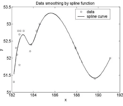
[image:11.612.160.410.280.495.2]In what follows, we consider some observed data, taken from [6], and we smooth these data by CV based smoothing spline function. The data, (xi, yi), i = 1,15, used in this application, represent the observed values for gas productivity and feedstock flow, in a cracking process, over 15 days. By applying the algorithm 1, based on the CV method, we obtain a value for the smoothing patrameter, equal to λCV = 0.0102, that indicates a good closeness to data . The following figure is the plot of the data together with the spline estimator.
Figure 4.1
with spline curve to the data. By contrary, if we suppose that the data are very noisy, we can choose a greater value, to obtain more smoothness for the estimator.
4. Some extensions of smoothing spline model
Certainly, at the same time with the notion of spline functions and al-though with the large variety of related practical problems, the notion of smoothing spline estimator bears a lot of extensions among which we remind in this paper the case of the models with bounded linear observational func-tionals and with the estimator searched in reproducing kernel Hilbert spaces (see the papers: [10], [11]). Also, we consider the case of models with data proceeded from multiple sources ([1], [2], [5]).
Spline smoothing in reproducing kernel Hilbert spaces. Smooth-ing Lg-spline estimators
This problem starting with the assumption of searching for smoothing spline estimator in reproducing kernel Hilbert spaces (definition (1.8)). Then in general, the estimator doesn’t keep the piecewise polynomial structure anymore, but it maintains the titulature of spline, being a solution to a certain variational problem, another facet of a spline function.
We consider the observational model, based on the data (xi, yi), i= 1, n,
yi =Lif +ǫi, i= 1, n (4.1)
with ǫ = (ǫ1, ǫ2, ..., ǫn)′ ∼ N(0, σ2I and Li, bounded linear functionals, on
HR, the reproducing kernel Hilbert space of real-valued functions onI, with reproducing kernel R.
Definition 4.1. We call the smoothing Lg-spline (nonparametric) regres-sion model, the model (4.1), for which we search for the estimator of f , by searching for f ∈HR, based on the criteria
min j
(
n−1
n
X
i=1
(yi−Lif)2+λkP1fk2HR )
where P1f is the orthogonal projection of f onto H1, in HR = H0 ⊕H1,
dim(H0) = M ≤ n. Such an estimator is called the smoothing Lg-spline function, λ being the related smoothing parameter.
Remark 4.2. IfI = [a, b], HR =Hm,2[a, b], the observational function-als, Li, i = 1, n, are the evaluation functionals defined by Lif = f(xi) and
Jm(f) = b
R
a
f(m)(x)2dx, then the Lg-spline smoothing problem is reduced to the (polynomial) spline smoothing problem presented in the previous section. The next theorem gives, under certain conditions, the existence and uniqueness of the Lg-spline estimator and also gives a characterization of this estimator. The related demonstration can be found in [10].
Theorem 4.3. Let φ1, φ2, ..., φM, span the null space H0 of P1 and let T be then×M matrix, defined byT ={Liφk}i=1,n, k=1,M. If T is of full column rank (equal to M), then the smoothing Lg-spline estimator, fλ, is uniquely given by
fλ = M
X
k=1
dkφk+ n
X
k=1
ciξi (4.3)
whereξi =P1ηi, d= (d1, d2, ..., dM)′ = (T′S−1T)− 1
T′S−1y,c= (c
1, c2, ..., cn)′ =
S−1I−T(T′S−1T)−1
T′S−1y, S = Σ + nλI,Σ = {(ξ
i, ξj)}i,j=1,n and
ηi ∈HR, is the representer of the bounded linear functional, Li.
Remark 4.4. i)The form (4.3) of the estimator reduces the Lg-spline smoothing problem to searching for c∈Rn and d ∈RM, that minimizes the expression
1
nky−(Σc+T d)k
2
+λc′Σc. (4.4)
ii)The cross validation function related to the Lg-spline smoothing prob-lem, that by minimizing in respect with λ, gives an estimator of the smooth-ing parameter, is
CV(λ) =n−1 n
X
k=1
yk−Lkfλ(−k)
2
wherefλ(−k)is the unique solution of the Lg-spline smoothing problem, stated for the data sample from which it was leaving out the k-th data.
Spline smoothing in the case of data from multiple sources with different weights
In this section, we have treated an extension of the spline data smoothing problem, namely, the model with data provided from more sources, for which the variances are different. The case of two sources with the same volume of data, related to functions defined on circle, was study in [5].
After the statement of the problem, we are concerned with the construc-tion of a selecconstruc-tion criteria for both the smoothing parameter and the relative weights corresponding to the sources. We begin with the regression model
Y =f(X) +ǫ (4.6)
for which, those n = N1 +N2 +...+Nl observations come from l sources, with different unknown acccuracies. We search for the estimator off in the space Hm,2[0,1]. In this case, we deal with l observational models,
y1i =f(x1i) +ǫ1i, i= 1, N1,
y2i =f(x2i) +ǫ2i, i= 1, N2,
...
yli =f(xli) +ǫli, i= 1, Nl, (4.7) with the errors, ǫj = (ǫj1, ǫj2, ..., ǫjNj)′ ∼ N(0, σ
2
jI). From those l sources, we have extracted Nj, j = 1, l, observations, materialized in the data yj = (yj1, ..., yjNj)′ and xj = xj1, ..., xjNj
′
, each of such observational models being homoscedastic, that is, the data from the same sources have the same variance. If we knew the variances, σ2
1 n " 1 σ2 1 N1 X i=1
(y1i −f(x1i))2+ 1 σ2 2 N2 X i=1
(y2i−f(x2i))2+...+ 1 σ2 l Nl X i=1
(yli−f(xli))2
#
+λJ(f) (4.8)
where J(f) = 1
R
0
f(m)(x)2dx.
It can be observed that the expression (4.8) is likewise the penalized least squares expression (3.1), with the mention that for each group of data we gave an importance directly proportional with the accuracy of the related source. This accuracy is obviously, invers proportional with the source vari-ance (under the hypothesis of l homoscedastic models).
From the computational point of view, an appropriate solution to the minimization problem corresponding to (4.8), consists in searching for f in a subspace of Hm,2[0,1], such that we can write
f ∼= N
X
k=1
ckBk (4.9)
whereBk,k = 1, N are the basis functions that span the disscused subspace. Such a subspace is S2m−1(∆), the space of 2m −1 degree, natural spline functions, associated with a partition ∆, with N knots, and an appropriate basis is that which contains among those N basis functions, N − 2m, B -spline functions, about which we know that they have a compact support (see theorem 1.6). In this case, we consider the partition ∆ of the interval [0,1], formed with all those n values xji, i = 1, Nj, j = 1, l, arranged in increasing order. Consequently, the problem of estimation forf ∈Hm,2[0,1] is reduced to the problem of estimation forf ∈S2m−1(∆), that is the problem of estimation for c∈Rn,c= (c1, c2, ..., cn)′.
If we replace (4.9) in the observational models (4.7) and use the matriceal writing, then we have l matriceal models,
y1 =B1c+ǫ1,
yl=Blc+ǫl,
with the errors, ǫj ∼N(0, σj2I), j = 1, l the matricesBj, j = 1, l, being given by
B1 = (Bik)1≤i≤N1 1≤k≤n
;Bik =Bk(x1i),
B2 = (Bik)1≤i≤N2 1≤k≤n
;Bik =Bk(x2i),
...
Bl = (Bik)1≤i≤Nl
1≤k≤n
;Bik =Bk(xli).
With these notations, we can prove the next propozition (see [1]):
Propozition 4.5. i) The solution to the variational problem based on the minimization of the expression (4.8), is given by the function f =
n
P
k=1
ckBk,
where csatisfies the variational problem,
min c∈Rn
r1ky1−B1ck2+r2ky2−B2ck2+...+rlkyl−Blck2+αc′Ωc (4.11) withα, the resulted smoothing parameter,θ, a nuisance parameter andrj, j = 1, l, the weighting parameters, given by the relations
α=σ1σ2...σl·λ·n,
θ =σ1σ2...σl,
rj =
σ1σ2...σj−1σj+1...σl
σj
, j = 1, l (4.12)
and with the matrix Ω =
R1
0
Bk(m)(x)Bs(m)(x)dx
ii) For fixed α > 0 and r = (r1, r2, ..., rl)′ ∈ Rl, the solution to the variational problem (4.11) is
cr,α = (r1B1′B1+r2B2′B2+...+rlBl′Bl+αΩ)− 1
(r1B1′y1+...+rlBl′yl) (4.13) We can observe that the estimator depends on the smoothing parameter
α, and the estimation of the ratios rj, j = 1, l, defined by (4.12). Beyond the implication of r in the full estimation of c, respectively of f, the estimation of r is important in itself, since it gives information regarding the relative accuracy of various sources (instruments), from the data are taken. In order to constructe a CV function for estimation of these parameters, we make the following notations:
Notations 4.6. In order to unify the parts corresponding to those l
sources, we will use the following notations:
y= (y′
1, y2′, ..., yl′)
′, B = (B′
1, B2′, ..., Bl′) ′,
I(r) =
1
√r1IN1 0 0 0 ... 0 0
0 √1r2IN2 0 0 ... 0 0
... ... ... ... ... ... ...
0 0 0 0 ... √r1
l−1INl−1 0
0 0 0 0 ... 0 √r1r2...rl−1INl
M = (r1B1′B1+r2B2′B2+...+rlBl′Bl+αΩ),
yr =I−1(r)
·y, Br =I−1(r)
·B.
Also, we denote byc(r,α−k), the spline estimator obtained as a solution to the variational problem (4.11) applied on the sample withn=N1+N2+...+Nl data, from which thek-th data was left out. Also, byyk, we denote the k-th element of the vector y, and by Bk and Bk,r, the k-th row of the matrix B, respectively Br.
Definition 4.7. The cross validation function related to the multiple sources spline smoothing problem, that by minimizing in respect withαandr, gives an estimator of the smoothing parameter and of the relative accuracies parameter, is
CV(r, α) = 1
n
n
X
k=1
yk−Bkc(r,α−k)
2
(4.14)
where c(r,α−k) is the unique solution of the spline smoothing problem (4.11), stated for the data sample from which it was leaving out the k-th data.
The minimization of this function, made in the purpose of the data driven estimation of r and α, represents an extension of the single source related criteria from (3.2) based on cross-validation method.
Obviously this problem can be written also, in the more general context of Lg-spline functions. Moreover, besides of these two extensions of a smoothing spline problem, presented here, a lot of extensions can be done in respect with problems that arise in practical context. We remind here only, the case of thin plate spline, the case of exponential data, partial spline models, the case of nonlinear observational functional and so on (see [10]).
References
[1].Breaz N., On the smoothing parameter in case of data from multiple sources, Acta Universitatis Apulensis, Mathematics-Informatics, Proc. of Int. Conf. on Theory and Appl. of Math. and Inf., Alba Iulia, no. 6, Part A, 75-84, 2003.
[2] Breaz N., Modele de regresie bazate pe funct¸ii spline, Presa Universi-tar˘a Clujean˘a, 2007.
[3].Craven P., Wahba G., Smoothing noisy data with spline functions: estimating the correct degree of smoothing by the method of generalized cross-validation, Numer. Math., 31, 377-403, 1979.
[4].Eubank R.L.,Nonparametric Regression and Spline Smoothing-Second Edition, Marcel Dekker, Inc., New York, Basel, 1999.
[6].Marinoiu C., Choosing a smoothing parameter for a curve fitting by
minimizing the expected prediction error, Acta Universitatis Apulensis, Mathematics-Informatics, no 5, 91-96, 2003.
[7].Micula Gh., Micula S., Handbook of Splines, Kluwer Academic Pub-lishers, Dordrecht-Boston-London, 1999.
[8].Schoenberg I.J.,Contribution to the problem of approximation of equidis-tant data by analytic functions, Parts A and B, Quart. Appl. Math. no. 4, 45-88, 112-441, 1946.
[9].Wahba G., Smoothing noisy data by spline functions, Numer. Math., 24, 383-393, 1975.
[10].Wahba G., Spline Models for Observational Data, Society for Indus-trial and Applied Mathematics, Philadelphia, 1990.
[11].Wahba G.,An Introduction to Model Building With Reproducing Ker-nel Hilbert Spaces, Tech. Report 1020, Univ of Wisconsin, Madison, 2000.
Authors:
Nicoleta Breaz
Department of Mathematics
”1 Decembrie 1918” University of Alba Iulia, str. N. Iorga, No. 11-13, 510009,
Alba, Romania,
e-mail: nbreaz@uab.ro Mihaela Aldea
Department of Mathematics
”1 Decembrie 1918” University of Alba Iulia, str. N. Iorga, No. 11-13, 510009,
Alba, Romania,