El e c t ro n ic
Jo ur
n a l o
f P
r o
b a b il i t y
Vol. 16 (2011), Paper no. 18, pages 504–530. Journal URL
http://www.math.washington.edu/~ejpecp/
Mirror coupling of reflecting Brownian motion
and an application to Chavel’s conjecture
∗
Mihai N. Pascu
∗Faculty of Mathematics and Computer Science
Transilvania University of Bra¸sov
Bra¸sov – 500091, Romania
[email protected]
http://cs.unitbv.ro/~pascu
Abstract
In a series of papers, Burdzy et al. introduced themirror couplingof reflecting Brownian motions in a smooth bounded domainD⊂Rd, and used it to prove certain properties of eigenvalues and
eigenfunctions of the Neumann Laplaceian onD.
In the present paper we show that the construction of the mirror coupling can be extended to the case when the two Brownian motions live in different domainsD1,D2⊂Rd.
As applications of the construction, we derive a unifying proof of the two main results concerning the validity of Chavel’s conjecture on the domain monotonicity of the Neumann heat kernel, due to I. Chavel ([12]), respectively W. S. Kendall ([16]), and a new proof of Chavel’s conjecture for domains satisfying the ball condition, such that the inner domain is star-shaped with respect to the center of the ball.
Key words:couplings, mirror coupling, reflecting Brownian motion, Chavel’s conjecture. AMS 2000 Subject Classification:Primary 60J65, 60H20; Secondary: 35K05, 60H3. Submitted to EJP on April 16, 2010, final version accepted January 26, 2011.
1
Introduction
The technique of coupling of reflecting Brownian motions is a useful tool, used by several authors in connection to the study of the Neumann heat kernel of the corresponding domain (see[2],[3],
[6],[11],[16],[17], etc).
In a series of paper, Krzysztof Burdzy et al. ([1],[2],[3],[6],[10],) introduced themirror coupling
of reflecting Brownian motions in a smooth domainD⊂Rdand used it in order to derive properties
of eigenvalues and eigenfunctions of the Neumann Laplaceian onD.
In the present paper, we show that the mirror coupling can be extended to the case when the two reflecting Brownian motions live in different domainsD1,D2⊂Rd.
The main difficulty in the extending the construction of the mirror coupling comes from the fact that the stochastic differential equation(s) describing the mirror coupling has a singularity at the
times when coupling occurs. In the case D1 = D2 = D considered by Burdzy et al. this problem
is not a major problem (although the technical details are quite involved, see[2]), since after the
coupling time the processes move together. In the case D1 6= D2 however, this is a major problem:
after the processes have coupled, it is possible for them to decouple (for example in the case when the processes are coupled and they hit the boundary of one of the domains).
It is worth mentioning that the method used for proving the existence of the solution is new, and it relies on the additional hypothesis that the smaller domain D2 (or more generally D1∩D2) is a convex domain. This hypothesis allows us to construct an explicit set of solutions in a sequence of
approximating polygonal domains forD2, which converge to the desired solution.
As applications of the construction, we derive a unifying proof of the two most important results on
the challenging Chavel’s conjecture on the domain monotonicity of the Neumann heat kernel ([12],
[16]), and a new proof of Chavel’s conjecture for domains satisfying the ball condition, such that the inner domain is star-shaped with respect to the center of the ball. This is also a possible new line of approach for Chavel’s conjecture (note that by the results in[4], Chavel’s conjecture does not hold in its full generality, but the additional hypotheses under which this conjecture holds are not known at the present moment).
The structure of the paper is as follows: in Section 2 we briefly describe the construction of Burdzy
et al. of the mirror coupling in a smooth bounded domainD⊂Rd.
In Section 3, in Theorem 3.1, we give the main result which shows that the mirror coupling can be
extended to the case when D2 ⊂ D1 are smooth bounded domains in Rd and D2 is convex (some
extensions of the theorem are presented in Section 5).
Before proceeding with the proof of theorem, in Remark 3.4 we show that the proof can be reduced to the case whenD1=Rd. Next, in Section 3.1, we show that in the caseD2= (0,∞)⊂D1=Rthe solution is essentially given by Tanaka’s formula (Remark 3.5), and then we give the proof of the main theorem in the 1-dimensional case (Proposition 3.6).
In Section 3.2, we first prove the existence of the mirror coupling in the case whenD2is a half-space
in Rd and D1 = Rd (Lemma 3.8), and then we use this result in order to prove the existence of
the mirror coupling in the case whenD2 is a polygonal domain inRd and D1=Rd (Theorem 3.9).
In Section 4 we give the proof of the main Theorem 3.1. The idea of the proof is to construct a sequence Ytn,Xt
of mirror couplings in Dn,Rd
, where Dn ր D2 is a sequence of convex
polygonal domains in Rd. Then, using the properties of the mirror coupling in convex polygonal
domains (Proposition 3.10), we show that the sequenceYtn converges to a process Yt, which gives
the desired solution to the problem.
The last section of the paper (Section 5) is devoted to the applications and the extensions of the mirror coupling constructed in Theorem 3.1.
First, in Theorem 5.3 we use the mirror coupling in order to give a simple, unifying proof of the results of I. Chavel and W. S. Kendall on the domain monotonicity of the Neumann heat kernel (Chavel’s Conjecture 5.1). The proof is probabilistic in spirit, relying on the geometric properties of the mirror coupling.
Next, in Theorem 5.4 we show that Chavel’s conjecture also holds in the more general case when one can interpose a ball between the two domains, and the inner domain is star-shaped with respect to the center of the ball (instead of being convex). The analytic proof given here is parallel to the geometric proof of the previous theorem, and it can also serve as an alternate proof of it.
Without giving all the technical details, we discuss the extension of the mirror coupling to the case of
smooth bounded domainsD1,2⊂Rd with non-tangential boundaries, such that D1∩D2 is a convex
domain.
The paper concludes with a discussion of the non-uniqueness of the mirror coupling. The lack of uniqueness is due to the fact that after coupling the processes may decouple, not only on the boundary of the domain, but also when they are inside the domain.
The two basic solutions give rise to thesticky, respectivelynon-stickymirror coupling, and there is a whole range of intermediate possibilities. The stickiness refers to the fact that after coupling the processes “stick” to each other as long as possible (“sticky” mirror coupling, constructed in Theorem 3.1), or they can immediately split apart after coupling (“non-sticky” mirror coupling), the general case (weak/mildmirror coupling) being a mixture of these two basic behaviors.
We developed the extension of the mirror coupling having in mind the application to Chavel’s conjec-ture, for which the sticky mirror coupling is the “right” tool, but perhaps the other mirror couplings (the non-sticky and the mild mirror couplings) might prove useful in other applications.
2
Mirror couplings of reflecting Brownian motions
Reflecting Brownian motion in a smooth domainD⊂Rdcan be defined as a solution of the
stochas-tic differential equation
Xt= x+Bt+ Z t
0
νD Xsd LsX, (2.1)
whereBt is ad-dimensional Brownian motion,νDis the inward unit normal vector field on∂Dand
LXt is the boundary local time of Xt (the continuous non-decreasing process which increases only
whenXt∈∂D).
In[1], the authors introduced themirror couplingof reflecting Brownian motion in a smooth domain
D⊂Rd (piecewiseC2 domain inR2 with a finite number of convex corners or aC2 domain inRd,
They considered the following system of stochastic differential equations:
Xt = x+Wt+ Z t
0
νD Xs
d LsX (2.2)
Yt = y+Zt+ Z t
0
νD Xsd LsY (2.3)
Zt = Wt−2
Z t
0
Ys−Xs
Ys−Xs2
Ys−Xs·dWs (2.4)
for t < ξ, whereξ = infs>0 :Xs=Ys is the coupling time of the processes, after which the
processesX andY evolve together, i.e.Xt=Yt andZt=Wt+Zξ−Wξfort≥ξ.
In the notation of[1], considering the Skorokhod map
Γ:C[0,∞):Rd→C[0,∞):D,
we haveX = Γ (x+W),Y = Γ y+Z, and therefore the above system is equivalent to
Zt= Z t∧ξ
0
GΓ y+Zs−Γ (x+W)sdWs+1t≥ξWt−Wξ, (2.5)
whereξ=inf¦s>0 :Γ (x+W)s= Γ y+Zs©. In[1]the authors proved the pathwise uniqueness and the strong existence of the processZt in (2.5) (given the Brownian motionWt).
In the aboveG:Rd→ Md×d denotes the function defined by
G(z) = (
H z
kzk
, ifz6=0
0, ifz=0 , (2.6)
where for a unitary vector m∈Rd, H(m) represents the linear transformation given by the d×d
matrix
H(m) =I−2m m′, (2.7)
that is
H(m)v=v−2(m·v)m (2.8)
is the mirror image ofv∈Rd with respect to the hyperplane through the origin perpendicular tom
(m′denotes the transpose of the vectorm, vectors being considered as column vectors).
The pair Xt,Ytt≥0 constructed above is called amirror couplingof reflecting Brownian motions in
Dstarting at(x,y)∈D×D.
Remark2.1. The relation (2.4) can be written in the equivalent form
d Zt=G Xt−YtdWt,
which shows that for t < ξ the increments of Zt are mirror images of the increments ofWt with
3
Extension of the mirror coupling
The main contribution of the author is the observation that the mirror coupling introduced above can be extended to the case when the two reflecting Brownian motion have different state spaces,
that is when Xt is a reflecting Brownian motion in a domain D1 and Yt is a reflecting Brownian
motion in a domain D2. Although the construction can be carried out in a more general setup (see
the concluding remarks in Section 5), in the present section we will consider the case when one of the domains is strictly contained in the other.
The main result is the following:
Theorem 3.1. Let D1,2⊂Rd be smooth bounded domains (piecewise C2-smooth boundary with convex corners inR2, or C2-smooth boundary inRd, d≥3will suffice) with D2⊂D1and D2 convex domain, and let x∈D1and y∈D2 be arbitrarily fixed points.
Given a d-dimensional Brownian motion Wt
t≥0starting at0on a probability space(Ω,F,P), there exists a strong solution of the following system of stochastic differential equations
Xt = x+Wt+ Z t
0
νD1 Xs
d LsX (3.1)
Yt = y+Zt+ Z t
0
νD
2 Ys
d LYs (3.2)
Zt = Z t
0
G Ys−Xs
dWs (3.3)
or equivalent
Zt= Z t
0
GeΓ y+Zs−Γ (x+W)sdWs, (3.4)
whereΓandΓedenote the corresponding Skorokhod maps which define the reflecting Brownian motion X = Γ (x+W) in D1, respectively Y =eΓ y+Z
in D2, and G :Rd → Md×d denotes the following
modification of the function G defined in the previous section:
G(z) = (
H
z
kzk
, if z6=0
I, if z=0 . (3.5)
Remark3.2. As it will follow from the proof of the theorem, with the choice ofG above, the solution
of the equation (3.4) in the case D1 = D2 = D is the same as the solution of the equation (2.5)
considered by the authors in[1](as also pointed out by the authors, the choice ofG(0)is irrelevant in this case).
Therefore, the above theorem is a natural generalization of the mirror coupling to the case when the two processes live in different spaces. We will refer to a solution(Xt,Yt)given by the above theorem
as amirror couplingof reflecting Brownian motions in(D1,D2)starting from x,y∈D1×D2, with
driving Brownian motionWt.
the coupling: once the processesXtandYt have coupled, they can either move together until one of them hits the boundary (sticky mirror coupling- this is in fact the solution constructed in the above theorem), or they can immediately split apart after coupling (non-sticky mirror coupling), and there is a whole range of intermediate possibilities (see the discussion at the end of Section 5).
As an application, in Section 5 we will use the former mirror coupling to give a unifying proof
of Chavel’s conjecture on the domain monotonicity of the Neumann heat kernel for domains D1,2
satisfying the ball condition, although the other possible choices for the mirror coupling might prove useful in other contexts.
Before carrying out the proof, we begin with some preliminary remarks which will allow us to reduce the proof of the above theorem to the caseD1=Rd.
Remark3.3. The main difference from the case whenD1=D2=Dconsidered by the authors in[1]
is that after the coupling timeξthe processes Xt andYt may decouple. For example, ift ≥ξis a
time whenXt =Yt∈∂D2, the processYt (reflecting Brownian motion inD2) receives a push in the
direction of the inward unit normal to the boundary of D2, while the processXt behaves like a free Brownian motion near this point (we assumed thatD2is strictly contained inD1), and therefore the
processes X andY will drift apart, that is they willdecouple. Also, as shown in Section 5, because the functionGhas a discontinuity at the origin, it is possible that the solutions decouple even when
they are inside the domainD2. This shows that without additional assumptions, the mirror coupling
is not uniquely determined (there is no pathwise uniqueness of (3.4)).
Remark 3.4. To fix ideas, for an arbitrarily fixed ǫ > 0 chosen small enough such that ǫ < dist ∂D1,∂D2, we consider the sequence ξnn≥1 of coupling times and the sequence τnn≥0
of times when the processes areǫ-decoupled (ǫ-decoupling times, or simplydecoupling timesby an
abuse of language) defined inductively by
ξn = inft> τn−1:Xt=Yt , n≥1,
τn = inft> ξn:kXt−Ytk> ǫ , n≥1,
whereτ0=0 andξ1=ξis the first coupling time.
To construct the general mirror coupling (that is, to prove the existence of a solution to (3.1) – (3.3) above, or equivalent to (3.4)), we proceed as follows.
First note that on the time interval [0,ξ], the arguments used in the proof of Theorem 2 in [1]
(pathwise uniqueness and the existence of a strong solutionZ of (3.4)) do not rely on the fact that
D1=D2, hence the same arguments can be used to prove the existence of a strong solution of (3.4) on the time interval[0,ξ1] = [0,ξ]. Indeed, givenWt, (3.1) has a strong solution which is pathwise
unique (the reflecting Brownian motionXt inD1), and therefore the proof of pathwise uniqueness
and the existence of a strong solution of (3.4) is the same as in[1]considering D= D2. Also note that as also pointed out by the authors, the valueG(0)is irrelevant in their proof, since the problem is constructing the processes until they meet, that is forYt−Xt 6=0, for which their definition ofG
is the same as in (3.5).
We obtain therefore the existence of a strong solutionZtto (3.4) on the time interval[0,ξ1]. By this we understand that the process Z verifies (3.4) for all t ≤ξ1 andZt isFt measurable for t ≤ξ1, where(Ft)t≥0 denotes the corresponding filtration of the driving Brownian motionWt.
[0,T]as follows. Considerξ1T =ξ1∧T, and note that ifZsolves (3.4), then
By the uniqueness results on the Skorokhod map (in the deterministic sense), we have
e
1 is a Brownian motion starting at the origin, with corresponding
filtrationFse =σ
independent ofFξT
1.
which is the same as the equation (3.4) for eZ, with the initial points x,y of the coupling replaced byYξT
1 =Γ(e y+Z)ξT1, respectivelyXξ1T = Γ(x+W)ξ1T, and the Brownian motionW replaced byWf.
If we assume the existence of a strong solution Zet of (3.6) until the first ǫ-decoupling time, by
patchingZ andeZwe obtain that
Zt1t≤ξT can apply again the results in[1](with the Brownian motionWτT
1+t−WτT1 instead ofWt, and the
starting points of the couplingXτT
1 andYτ
T
1 instead of x and y) in order to obtain a strong solution
of (3.4) until the first coupling time. By patching we obtain the existence of a strong solution of (3.4) on the time interval0,ξT2.
Proceeding inductively as indicated above, since only a finite number of coupling/decoupling times
ξn and τn can occur in the time interval[0,T], we can construct a strong solution Z to (3.4) on the time interval[0,T]for anyT>0 (and therefore on[0,∞)), provided we show the existence of strong solutions of equations of type (3.6) until the firstǫ-decoupling time.
In order to prove this claim, since Γ(e y +Z)ξT
1 and Γ (x+W)ξ
T
1 are Fξ
T
1 measurable and the
σ-algebra FξT
1 is independent of the filtrationFe = (Fte)t≥0 of the driving Brownian motionWft, it
suffices to show that for any starting points x= y ∈D2 of the mirror coupling, there exists a strong
solution of (3.4) until the firstǫ-decoupling timeτ1. Sinceǫ <dist ∂D1,∂D2
processXt cannot reach the boundary∂D1 before the firstǫ-decoupling timeτ1, and therefore we
can consider thatXt is a free Brownian motion inRd, that is, we can reduce the proof of Theorem
3.1 to the case when D1=Rd.
We will give the proof of the Theorem 3.1 first in the 1-dimensional case, then we will extend it to the case of polygonal domains inRd, and we will conclude with the proof in the general case.
3.1
The
1-dimensional case
From Remark 3.4 it follows that in order to construct the mirror coupling in the 1-dimensional case, it suffices to considerD1=RandD2= (0,a), and to show that for an arbitrary choice x ∈[0,a]of
the starting point of the mirror coupling,ǫ∈(0,a)sufficiently small and Wtt≥0 a 1-dimensional Brownian motion starting atW0=0, we can construct a strong solution on[0,τ1]of the following system
Xt = x+Wt (3.7)
Yt = x+Zt+LYt (3.8)
Zt = Z t
0
G Ys−XsdWs (3.9)
where τ1 = infs>0 :|Xs−Ys|> ǫ is the first ǫ-decoupling time and the function G :
R→ M1×1≡Ris given in this case by
G(x) = ¨
−1, if x 6=0
+1, if x =0 . (3.10)
Remark 3.5. Before proceeding with the proof, it is worth mentioning that the heart of the
con-struction is Tanaka’s formula. To see this, consider for the momenta = ∞, and note that Tanaka
formula
x+Wt=x+ Z t
0
sgn x+WsdWs+L0t(x+W)
gives a representation of the reflecting Brownian motionx+Wt
in which the increments of the
martingale part ofx+Wt
are the increments ofWtwhenx+Wt∈[0,∞), respectively the opposite
(minus) of the increments ofWt in the other case (L0t(x+W) denotes here the local time at 0 of
x+Wt).
Since x +Wt ∈[0,∞) is the same asx+Wt= x +Wt, from the definition of the function G it follows that the above can be written in the form
x+Wt
=x+
Z t
0
Gx+Ws
− x+Ws
dWs+Lxt+W,
which shows that a strong solution to (3.7) – (3.9) above (in the casea=∞) is given explicitly by
Xt=x+Wt,Yt=x+WtandZt=R0tsgn x+WsdWs.
Proposition 3.6. Given a 1-dimensional Brownian motion Wtt≥0 starting at W0 = 0, a strong
From (3.11) and the definition (3.10) of the functionG we obtain
sgn x+Ws
and therefore the previous formula can be written equivalently
3.2
The case of polygonal domains
In this section we will consider the case when D2 ⊂ D1 ⊂ Rd are polygonal domains (domains
bounded by hyperplanes in Rd). From Remark 3.4 it follows that we can consider D1 = Rd and
therefore it suffices to prove the existence of a strong solution of the following system
Xt = X0+Wt (3.12)
Yt = Y0+Zt+ Z t
0
νD2 Ysd LYs (3.13)
Zt = Z t
0
G Ys−XsdWs (3.14)
or equivalently of the equation
Zt= Z t
0
GΓe Y0+Z
s−X0−Ws
dWs, (3.15)
whereWt is ad-dimensional Brownian motion starting atW0=0 andX0=Y0∈D2.
The construction relies on the following skew product representation of Brownian motion in spher-ical coordinates:
Xt=RtΘσ
t, (3.16)
where Rt = kXtk ∈ BES(d) is a Bessel process of order d andΘt ∈BMSd−1 is an independent Brownian motion on the unit sphereSd−1inRd, run at speed
σt= Z t
0
1
R2sds, (3.17)
which depends only onRt.
Remark3.7. One way to construct the Brownian motionΘt = Θtd−1 on the unit sphereSd−1 ⊂Rd
is to proceed inductively on d ≥2, using the following skew product representation of Brownian
motion on the sphereΘdt−1∈Sd−1(see[15]):
Θdt−1=cosθt1, sinθt1Θdα−2
t
,
where θ1 ∈ LEG(d−1) is a Legendre process of order d−1 on [0,π], and Θd−2
t ∈Sd−2 is an
independent Brownian motion onSd−2, run at speed
αt= Z t
0
1
sin2θ1
s
ds.
Therefore, ifθt1, . . .θtd−1are independent processes, withθi∈LEG(d−i)on[0,π]fori=1, . . . ,d−
2, andθtd−1is a 1-dimensional Brownian (note thatΘ1t =cosθt1, sinθt1∈S1is a Brownian motion onS1), Brownian motionΘdt−1on the unit sphereSd−1⊂Rd is given by
or by
Θtd−1=θt1, . . . ,θtd−2,θtd−1 (3.18)
in spherical coordinates.
To construct the solution of (3.12) – (3.14), we first consider the case when D2 is a half-space
Hd+=¦z1, . . . ,zd∈Rd:zd>0©.
Given an angleϕ∈R, we introduce the rotation matrixR ϕ∈ Md×d which leaves invariant the
firstd−2 coordinates and rotates clockwise by the angleαthe remaining 2 coordinates, that is
R(α) =
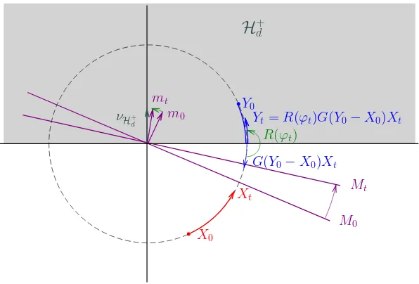
A strong solution of the system (3.12) – (3.14) is explicitly given by
Yt=
hyperplane through the origin perpendicular tom.
By Itô formula, we have
Xt
Yt=R(ϕt)G(Y0−X0)Xt
M0 Mt
X0 Y0
G(Y0−X0)Xt
H
+dνH+ d
m0 mt
R(ϕt)
Figure 1: The mirror coupling of a free Brownian motionXt and a reflecting Brownian motionYt in
the half-spaceHd+.
Note that the composition R◦G (a symmetry followed by a rotation) is a symmetry, and since
kYtk = kXtk for all t ≥ 0, it follows that Xt and Yt are symmetric with respect to a hyperplane
passing through the origin for all t ≤ξ. Therefore, from the definition (3.5) of the function G it
follows that we haveYt=G Yt−Xt
Xt for allt≤ξ.
Also note that whenLs0θed−1increases,Ys∈∂D2 and we have
R
ϕs+π
2
G Y0−X0Xs=R
π
2
Ys=νD
2 Ys
,
and ifLsπθed−1increases,Ys∈∂D2and we have
R
ϕs+π
2
G Y0−X0Xs=R
π
2
Ys=−νD2 Ys.
It follows that the relation (3.22) can be written in the equivalent form
Yt∧ξ=Y0+ Z t∧ξ
0
G Ys−Xsd Xs+ Z t∧ξ
0
νD
2 Ys
d LsY,
where LYt = L0tθed−1+Lπt θed−1 is a continuous non-decreasing process which increases only whenYt ∈∂D2, and thereforeYt given by (3.21) is a strong solution of the system (3.12) – (3.14) fort≤ξ.
For t≥ξ, we haveYt = Xt
d =
case, by Tanaka formula we obtain:
The process LYt = L0tXd in (3.23) is a continuous non-decreasing process which increases only whenYt ∈∂D2 (L0t
Xd represents the local time at 0 of the last cartesian coordinateXd ofX), which shows that Yt also solves (3.12) – (3.14) for t ≥ξ, and thereforeYt is a strong solution of (3.12) – (3.14) fort≥0, concluding the proof.
Consider now the case of a general polygonal domain D2 ⊂ Rd. We will show that a strong
so-lution of the system (3.12) – (3.14) can be constructed from the previous lemma by choosing the appropriate coordinate system.
Consider the times σn
n≥0 at which the solution Yt hits different bounding hyperplanes of∂D2,
that isσ0=infs≥0 :Ys∈∂D2 and inductively
σn+1=inf
¨
t≥σn:
Yt∈∂D2andYt,Yσn belong to different1
bounding hyperplanes of∂D2
«
, n≥0. (3.24)
If X0 = Y0 ∈ ∂D2 belong to a certain bounding hyperplane of D2, we can chose the coordinate
system so that this hyperplane isHd =¦z1, . . . ,zd∈Rd:zd=0©andD2⊂ Hd+, and we letHd
be any bounding hyperplane ofD2 otherwise.
By Lemma 3.8 it follows that on the time interval[σ0,σ1), the strong solution of (3.12) – (3.14) is given explicitly by (3.21).
If σ1 < ∞, we distinguish two cases: Xσ
1 = Yσ1 and Xσ1 6= Yσ1. Let H denote the bounding
hyperplane ofDwhich containsYσ1, and letνH denote the unit normal toH pointing inside D2.
If Xσ1 = Yσ1 ∈ H, choosing again the coordinate system conveniently, we may assume thatH is
the hyperplane isHd =¦z1, . . . ,zd∈Rd :zd=0©, and on the time interval[σ1,σ2)the coupling
system so that the condition (3.20) holds. IfYσ1−Xσ1 is a vector perpendicular toH, by choosing
1Since 2-dimensional Brownian motion does not hit points a.s., thed-dimensional Brownian motionY
t does not hit
the coordinate system so thatH =Hd=¦z1, . . . ,zd∈Rd:zd=0©, the problem reduces to the
1-dimensional case (the firstd−1 coordinates of X andY are the same), and it can be handled as
in Proposition 3.6 by the Tanaka formula. The proof being similar, we omit it.
IfXσ16=Yσ1∈ H andYσ1−Xσ1 is not orthogonal toH, considerXeσ1 =prH Xσ1 the projection of
Xσ1 ontoH, and therefore Xeσ1 6= Yσ1. The plane of symmetry of Xσ1 and Yσ1 intersects the line
determined byXeσ
1 and Yσ1 at a point, and we consider this point as the origin of the coordinate
system (note that the intersection cannot be empty, for otherwise the vectorsYσ1−Xσ1andYσ1−Xeσ1
were parallel, which is impossible since then Yσ1−Xσ1,Yσ1−Xeσ1 and Yσ1−Xeσ1,Xσ1−Xeσ1 were
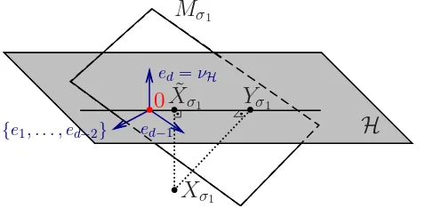
perpendicular pairs of vectors, contradictingXeσ16=Yσ1 – see Figure 2).
Yσ
1Xσ
1˜
X
σ1H
0
Mσ
1ed=νH
ed−1
{e1, . . . , ed−2}
Figure 2: Construction of the appropriate coordinate system.
Choose an orthonormal basis e1, . . . ,ed in Rd such that ed = νH is the normal vector to H
pointing inside D2, ed−1 = 1
kYσ1−Xσ1k
Yσ
1−Xσ1
is a unit vector lying in the 2-dimensional plane
determined by the origin and the vectors ed and Yσ
1−Xσ1, and
e1, . . . ,ed−2 is a completion of
ed−1,ed to an orthonormal basis inRd (see Figure 2).
Note that by the construction, the vectors e1, . . . ,ed−2 are orthogonal to the 2-dimensional
hyper-plane containing the origin and the pointsXσ1 andYσ1, and therefore Xσ1 and Yσ1 have the same (zero) first d−2 coordinates; also, since Xσ
1 and Yσ1 are at the same distance from the origin,
it follows that Yσ1 can be obtained from Xσ1 by a rotation which leaves invariant the first d−2
coordinates, which shows that the condition (3.20) of Lemma 3.8 is satisfied.
Since by construction the bounding hyperplane H of D2 at Yσ1 is given by Hd =
¦
z1, . . . ,zd∈Rd :zd =0© and D2 ⊂ Hd+ =
¦
z1, . . . ,zd∈Rd:zd>0©, we can apply Lemma
3.8 to deduce that on the time interval [σ1,σ2) a solution of (3.12) – (3.14) is given by
Xσ1+t,Yσ1+t
t∈[0,σ2−σ1).
Repeating the above argument we can construct inductively (in the appropriate coordinate systems) the solution of (3.12) – (3.14) on any time interval [σn,σn+1), n≥1, and therefore we obtain a
strong solution of (3.12) – (3.14) defined for t≥0.
We summarize the above discussion in the following:
Moreover, between successive hits of different bounding hyperplanes of D2 (i.e. on each time interval
[σn,σn+1) in the notation above), the solution is given by Lemma 3.8 in the appropriately chosen coordinate system.
We will refer to the solution Xt,Ytt≥0constructed in the previous theorem as amirror couplingof reflecting Brownian motions inRd,D2with starting pointX0=Y0∈D2.
If Xt 6= Yt, the hyperplane Mt of symmetry between Xt and Yt (the hyperplane passing through
Xt+Yt
2 with normal mt =
1
kYt−Xtk Yt−Xt
) will be referred to as the mirror of the coupling. For definiteness, whenXt=Yt we letMt denote any hyperplane passing through Xt=Yt, for example
we can chooseMt such that it is a left continuous function with respect to t.
In the particular case of a convex polygonal domainD2, some of the properties of the mirror coupling are contained in the following:
Proposition 3.10. If D2⊂Rd is a convex polygonal domain, for any X0=Y0∈D2, the mirror coupling given by the previous theorem has the following properties:
i) If the reflection takes place in the bounding hyperplaneH of D2 with inward unitary normal
νH, then the angle∠(mt;νH)decreases monotonically to zero.
ii) When processes are not coupled, the mirror Mt lies outside D2.
iii) Coupling can take place precisely when Xt∈∂D2. Moreover, if Xt∈D2, then Xt=Yt.
iv) If Dα ⊂ Dβ are two polygonal domains and (Ytα;Xt), (Y β
t ;Xt) are the corresponding mirror
coupling starting from x∈Dα, for any t>0we have
sup
s≤tk
Ysα−Ysβk ≤DistDα,Dβ:= max
xα∈∂Dα,xβ∈∂Dβ
(xβ−xα)·νDα(xα)≤0
kxα−xβk. (3.25)
Proof. i) In the notation of Theorem 3.9, on the time interval [σ0,σ1) we have Yt = Xt, so
∠ mt,νH
=0 and therefore the claim is verified in this case.
On an arbitrary time interval[σn,σn+1), in the appropriately chosen coordinate system,Yt is given
by Lemma 3.8. Fort< ξ,Ytis given by the rotationR ϕtofG Y0−X0Xt which leaves invariant the first(d−2)coordinates, and therefore
∠ mt,νH=∠ m0,νH+ L
0
t −L π t
2 ,
which proves the claim in this case (note that before the coupling time ξ only one of the
non-decreasing processesL0t and Lπt is not identically zero).
Since fort≥ξwe haveYt=Xt1, . . . ,Xtd, we have∠ mt,νH=0 which concludes the proof of the claim.
ii) On the time interval[σ0,σ1)the processes are coupled, so there is nothing to prove in this case.
On the time interval [σ1,σ2), in the appropriately chosen coordinate system we have
¦
z1, . . . ,zd∈Rd :zd =0© of D2 where the reflection takes place, and therefore Mt ∩D2 = ∅
in this case.
Inductively, assume the claim is true for t < σn. By continuity, Mσn∩D2=∅, thusD2 lies on one side ofMσn. By the previous proof, the angle∠ mt,νH
betweenmt and the inward unit normal
νH to bounding hyperplaneH ofD2where the reflection takes place decreases to zero. Since D2 is
a convex domain, it follows that on the time interval[σn,σn+1)we haveMt∩D2=∅, concluding
the proof.
iii) The first part of the claim follows from the previous proof (when the processes are not coupled, the mirror (henceXt) lies outsideD2; by continuity, it follows that at the coupling timeξwe must haveXξ=Yξ∈∂D2).
To prove the second part of the claim, consider an arbitrary time interval[σn,σn+1)between two successive hits ofYtto different bounding hyperplanes ofD2. In the appropriately chosen coordinate
system,Yt is given by Lemma 3.8. After the coupling timeξ,Yt is given byYt=Xt1, . . . ,Xtd, and therefore ifXt∈D2(thusXdt ≥0) we haveYt=X1t, . . . ,Xtd=Xt, concluding the proof.
iv) LetMtα andMtβ denote the mirrors of the coupling inDα, respectivelyDβ, with the same driving Brownian motionXt.
SinceYtα andXt are symmetric with respect to Mtα, and Ytβ and Xt are symmetric with respect to
Mβt, it follows that Ytβ is obtained from Ytβ by a rotation which leaves invariant the hyperplane
Mαt ∩Mtβ, or by a translation by a vector orthogonal to Mtα (in the case when Mtα and Mtβ are parallel).
The angle of rotation (respectively the vector of translation) is altered only when either Ytα or
Ytβ are on the boundary of Dα, respectively Dβ. Since Dα ⊂ Dβ are convex domains, the angle
of rotation (respectively the vector of translation) decreases when Ytβ ∈ Dβ or when Ytα ∈ ∂Dα
and
Ytβ−Ytα
·νDαYtα > 0 (in these cases Ytβ and Ytα receive a push such that the distance
kYtα−Ytβkis decreased), thus the maximum distance kYtα−Ytβk is attained whenYtα ∈∂Dα and
Ytβ−Ytα
·νDαYtα≤0, and the formula follows.
4
The proof of Theorem 3.1
By Remark 3.4, it suffices to consider the case when D1 = Rd and D2 ⊂ Rd is a convex bounded
domain with smooth boundary. To simplify the notation, we will drop the index and writeDforD2
in the sequel.
Let Dnn≥1 be an increasing sequence of convex polygonal domains in Rd with Dn ⊂ Dn+1 and
∪n≥1Dn=D.
ConsiderYtn,Xt
t≥0 a sequence of mirror couplings in
Dn,Rd with starting point x ∈ D1 and
driving Brownian motion Wtt≥0 withW0=0, given by Theorem 3.9.
By Proposition 3.10, for anyt>0 we have
sup
s≤t
Ysm−Ysn≤Dist Dn,Dm= max
xn∈∂Dn,xm∈∂Dm
(xm−xn)·νDn(xn)≤0
xn−xmn,m→
henceYtn converges a.s. in the uniform topology to a continuous processYt.
Since(Yn)n≥1 are reflecting Brownian motions in Dnn≥1 and Dn րD, the law of Yt is that of a
reflecting Brownian motion in D, that is Yt is a reflecting Brownian motion in Dstarting at x ∈D
(see [8]). Also note that since Ytn are adapted to the filtration FW = Ft
t≥0 generated by the
Brownian motionWt, so isYt.
By construction, the driving Brownian motionZtn ofYtnsatisfies
Ztn= Z t
0
GYtn−XtdWt, t≥0.
Consider the process
Zt= Z t
0
G Ys−Xs
dWs,
and note that sinceY isFW-adapted and||G||=1, by Lévy’s characterization of Brownian motion,
Zt is a freed-dimensional Brownian motion starting atZ0=0, also adapted to the filtrationFW.
We will show that Z is the driving process of the reflecting Brownian motion Yt, that is, we will
show that
Yt=x+Zt+LYt =x+ Z t
0
G Ys−Xs
dWs+LYt, t ≥0.
Note that the mapping z 7−→ G(z) is continuous with respect to the norm ||A|| =
ai j
=
Pd i,j=1a
2
i j of d ×d matrices at all points z ∈ R
d
− {0}, hence GYsn−Xs
→
n→∞ G Ys−Xs
if
Ys−Xs6=0. IfYs−Xs=0, then eitherYs=Xs∈DorYs=Xs∈∂D.
If Ys = Xs ∈ D, since Dn ր D, there exists N ≥ 1 such that Xs ∈ DN, hence Xs ∈ Dn for all
n≥N. By Proposition 3.10, it follows that Ysn =Xs for all n≥N, hence in this case we also have
GYsn−Xs=G(0) →
n→∞G(0) =G Ys−Xs
.
have:
since Yt is a reflecting Brownian motion in D, and therefore it spends zero Lebesgue time on the
boundary ofD.
Since||G||=1, using the above and the bounded convergence theorem we obtain
lim
and therefore by Doob’s inequality it follows that
Esup
By construction,Ztn is the driving Brownian motion forYtn, that is
Ytn=x+Ztn+
and passing to the limit withn→ ∞we obtain
It remains to show thatAt is a process of bounded variation. For an arbitrary partition 0=t0<t1<
whereσn is the surface measure on∂Dn, and the last inequality above follows from the estimates
in[5]on the Neumann heat kernels pD
n t,x,y
(see the remarks preceding Theorem 2.1 and the proof of Theorem 2.4 in[7]).
From the above it follows thatAt =Yt−x−Zt is a continuous,FW-adapted process (since Yt, Zt
are continuous,FW-adapted processes) of bounded variation.
By the uniqueness in the Doob-Meyer semimartingale decomposition of the reflecting Brownian motionYt inD, it follows that
At= Z t
0
νD Ysd LsY, t≥0,
where LY is the local time ofY on the boundary∂D. It follows that the reflecting Brownian motion
Yt inDconstructed above is a strong solution to
Yt=x+
or equivalent, the driving Brownian motionZt=
Rt
concluding the proof of Theorem 3.1.
5
Extensions and applications
As an application of the construction of mirror coupling, we will present a unifying proof of the two most important results on Chavel’s conjecture.
It is not difficult to prove that the Dirichlet heat kernel is an increasing function with respect to the
domain. Since for the Neumann heat kernel pD t,x,yof a smooth bounded domain D⊂Rd we
the monotonicity in the case of the Neumann heat kernel should be reversed.
Conjecture 5.1(Chavel’s conjecture,[12]). Let D1,2⊂Rd be smooth bounded convex domains inRd, d ≥ 1, and let pD1 t,x,y
, pD2 t,x,y
denote the Neumann heat kernels in D1, respectively D2. If D2⊂D1, then
pD
1 t,x,y
≤pD
2 t,x,y
, (5.1)
for any t≥0and x,y ∈D1.
Remark5.2. The smoothness assumption in the above conjecture is meant to insure the a.e. exis-tence of the inward unit normal to the boundaries ofD1andD2, that is the boundaries should have a locally differentiable parametrization. Requiring that the boundary of the domain is of classC1,α
(0< α <1) is a convenient hypothesis on the smoothness of the domainsD1,2.
In order to simplify the proof, we will assume that D1,2 are smooth C2 domains (the proof can be
extended to a more general setup, by approximatingD1,2by less smooth domains).
Among the positive results on Chavel conjecture, the most general known results (and perhaps the easiest to use in practice) are due to I. Chavel ([12]) and W. Kendall ([16]), and they show that if there exists a ball B centered at either x or y such that D2 ⊂ B⊂ D1, then the inequality (5.1) in
Chavel’s conjecture holds for anyt>0.
While there are also other positive results which suggest that Chavel’s conjecture is true for certain classes of domains (see for example[11],[14]), in[4]R. Bass and K. Burdzy showed that Chavel’s conjecture does not hold in its full generality (i.e. without additional hypotheses).
We note that both the proof of Chavel (the case when D1 is a ball centered at either x or y) and
Kendall (the case when D2 is a ball centered at either x or y) relies in an essential way that one
of the domains is a ball: the first uses an integration by parts technique, while the later uses a coupling argument of the radial parts of Brownian motion, and none of these proofs seem to be easily applicable to the other case.
Using the mirror coupling, we can derive a simple, unifying proof of these two important results, as follows:
Theorem 5.3. Let D2 ⊂ D1 ⊂Rd be smooth bounded domains and assume that D2 is convex. If for x,y ∈D2 there exists a ball B centered at either x or y such that D2⊂B ⊂D1, then for all t≥0we have
pD1 t,x,y≤pD2 t,x,y. (5.2)
Proof. Considerx,y ∈D2 arbitrarily fixed and assume thatD2⊂B=B y,R⊂D1 for someR>0.
By eventually approximating the convex domain D2 by convex polygonal domains, it suffices to
prove the claim in the case when D2 is a convex polygonal domain.
Let Xt,Yt
be a mirror coupling of reflecting Brownian motions in D1,D2
starting atx ∈D2. The
idea of the proof is to show that for all timest ≥0,Yt is at a distance from y is no greater than the
distance fromXt to y.
Lett0≥0 be a time when the processes are at the same distance from y, and let t1≥t0be the first time aftert0 when the processXt hits the boundary ofD1.
Note that by the ball condition we havekXt− yk=R >kYt−ykfor any t ≥0, and in particular this holds for t=t1. Since the processes Xt andYt are continuous, the distances fromXt andYt to
kYt−yk ≤ kXt−ykfor all t ∈[t0,t1]. Also note that on the time interval [t0,t1]the process Xt
behaves like a free Brownian motion.
We distinguish the following cases:
i) The processes are coupled at timet0 (i.e. Xt0=Yt0);
In this case, the distances from Xt and Yt to y will remain equal until the first time when the
processes hit the boundary of D2. Since on the time interval[t0,t1]the process Xt behaves like a
free Brownian motion, by Proposition 3.10 ii) it follows that when processes are not coupled, the mirrorMt of the coupling lies outside the domain D2. Since the domain D2 is assumed convex, this
shows in particular that the mirror Mt of the coupling cannot separate the points Yt and y, and
therefore the distance from Yt to y is smaller than or equal to the distance from Xt to y, for all
t∈[t0,t1].
ii) The processes are decoupled at timet0;
In this case, sinceYt0−y
=Xt0−y
andXt06=Yt0, the hyperplaneMt0of symmetry betweenXt0
andYt0passes through the point y, soMt0does not separate the pointsYt0 and y.
The processesXtandYt will remain at the same distance from y until the first time whenYt∈∂D2.
Since on the time interval[t0,t1]the processXt behaves like a free Brownian motion, by Theorem
3.9, it follows that between successive hits of different boundary hyperplanes of D2, the mirror
Mt of the coupling describes a rotation which leaves invariantd−2 coordinate axes. Moreover, by
Proposition 3.10 the rotation is directed in such a way that the angle∠(mt,νH)between the normal
mt= 1
kYt−Xtk Yt−Xt
ofMt and the inner normalνH of the bounding hyperplaneH ofD2 where
the reflection takes place decreases monotonically to zero (see Figure 1).
Since the hyperplaneMt0 does not separate the pointsYt0 and y, simple geometric considerations show that Mt will not separate the points Yt and y for all t ∈[t0,t1], and thereforekYt− yk ≤
kXt− ykfor allt∈[t0,t1], concluding the proof of the claim.
We showed that for any t≥0 we havekYt−yk ≤ kXt− yk, and therefore
Px kXt−yk< ǫ≤Px kYt−yk< ǫ,
for anyǫ >0 andt≥0.
Dividing the above inequality by the volume of the ballB y,ǫand passing to the limit withǫց0, from the continuity of the transition density of the reflecting Brownian motion in the space variable we obtain
pD1 t,x,y
≤pD2 t,x,y
, t≥0,
concluding the proof of the theorem.
As also pointed out by Kendall in[16], we note that in the above theorem the convexity of the larger domainD1is not needed in order to derive the validity of condition (5.1) in Chavel’s conjecture. We
can also replace the hypothesis on the convexity of the smaller domainD2by the weaker hypothesis
thatD2is a star-shaped domain with respect to either x or y, as follows:
Theorem 5.4. Let D2⊂ D1 ⊂Rd be smooth bounded domains. If for x,y ∈D2 there exists a ball B centered at either x or y such that D2⊂B⊂D1 and D2is star-shaped with respect to the center of the ball, then for all t≥0we have
pD1 t,x,y
≤pD2 t,x,y
Proof. We will present an analytic proof which parallels the geometric proof of the previous theorem.
Considerx,y ∈D2 arbitrarily fixed and assume thatD2⊂B=B y,R⊂D1 for someR>0 andD2
is a star-shaped domain with respect to y.
By eventually approximatingD2 with star-shaped polygonal domains, it suffices to prove the claim
in the case whenD2 is a polygonal star-shaped domain.
Let Xt,Yt
be a mirror coupling of reflecting Brownian motions in D1,D2
starting atx ∈D2. The
idea of the proof is to show that for all timest ≥0,Yt is at a distance from y is no greater than the distance fromXt to y.
We can reduce the proof to the case whenD1=Rd as follows. Consider the sequences of stopping
times(ξn)n≥1 and(τn)n≥1defined inductively by
τ0 = 0,
ξn = inft> τn−1:Xt∈∂D1 , n≥1,
τn = inft> ξn:kXt−yk=kYt−yk , n≥1.
Note that by the ball condition we have kXξn − yk > kYξn − yk for any n ≥ 1, and therefore
kXt− yk ≥ kYt−ykfor anyn≥1 and anyt∈
ξn,τn
. In order to prove that the same inequality holds on the intervalsτn,ξn+1
forn≥0, we proceed as follows.
On the set{τn<∞}, the pair(Xet,Yet) =Xτn+t,Yτn+t
defined fort≤ξn+1−τnis a mirror coupling
in(Rd,D2)with driving Brownian motionWft =Wτn+t−Wτn (and Zet= Zτn+t−Zτn), and starting points(Xe0,Ye0) = (Xτ
n,Yτn)independent of the filtration of Bet (see Remark 3.4). In order to prove the claim it suffices therefore to show that for any pointsu∈Rd andv∈D2withku−yk=kv−yk, the mirror coupling(Xt,Yt)in(Rd,D2)with starting points(X0,Y0) = (u,v)verifies
kXt−yk ≥ kYt− yk, t≥0. (5.4)
Consider therefore a mirror coupling (Xt,Yt) in (Rd,D2) with starting points(X0,Y0) = (u,v) ∈
Rd×D2satisfyingku−yk=kv−yk.
If u= v, from the construction of the mirror coupling it follows that Xt = Yt until the process Yt
hits the boundary of D2, and therefore the inequality in (5.4) holds for these values of t. After
the process Yt hits a bounding hyperplane of D2, by Lemma 3.8 it follows that in an appropriate
coordinate systemYt is given byYt= (X1t, . . . ,Xtd−1,|Xtd|), until the timeσwhen the processY hits
a different bounding hyperplane of D2, and therefore the inequality in (5.4) is again verified for
the corresponding values oft (in the chosen coordinate system we must have y = (y1, . . . ,yd)with
yd > 0, and therefore kXt−yk2− kYt− yk2 =2yd
|Xdt| −Xdt≥ 0). If at timeσ the processes are coupled (i.e.Xσ=Yσ∈∂D2), we can apply the above argument inductively, and find a timeσ1 when the processes are decoupled andkXt−yk ≥ kYt−ykfor allt≤σ1.
The above discussion shows that without loss of generality we may further reduce the proof of the claim to the case when(u,v)∈Rd×D2withu6=vandku−yk ≥ kv−yk. Also, the above discussion
The mirror coupling defined by (3.1) – (3.3) becomes in the case
whereG is given by (3.5). In order to prove the claim we will show that
Rt=kXt−yk2− kYt−yk2≥0, t ≤ζ, (5.8)
whereζis the first coupling time.
Using the Itô formula it can be shown that the processRtverifies the stochastic differential equation
Rt=R0−2
and therefore by Lévy’s characterization of Brownian motion it follows that eBt = Bα
t∧ζ is a
1-dimensional Brownian motion (possibly stopped at time ζ, if Aζ < ∞), where the time change
αt=inf{s≥0 :As>t}is the inverse of the nondecreasing processAt.
Since the polygonal domain D2 is assumed star-shaped with respect to the point y, geometric
con-siderations show that
(z− y)·νD
2(z)≤0, (5.12)
for all the pointsz∈∂D2for which the inside pointing normalνD2(z)at the boundary pointzofD2
is defined, that is for all pointsz∈∂D2 not lying on the intersection of two bounding hyperplanes
ofD2. Since the reflecting Brownian motionYt does not hit the set of these exceptional points with positive probability, we may assume that the above condition is satisfied for all points, and therefore
(Yes−y)·νD2(Yes)≤0 a.s, (5.13)
for all timess≥0 whenYes∈∂D2.
Since eLYt is a nondecreasing process of t ≥ 0, a standard comparison argument for solutions of
stochastic differential equations shows that the solutioneRt of (5.11) satisfiesRet ≥ρt for all t≥0, whereρt is the solution of the stochastic differential equation
ρt=Re0+ Z t
0