Reduce Divorce Rates?
A Reexamination
Bradley T. Heim
a b s t r a c t
During the 1990s, expenditures on Child Support Enforcement increased dramatically, as did the amount of money collected in these efforts. This paper examines whether there is a link between the Child Support En-forcement program and the divorce behavior of married couples with chil-dren. Previous work, notably that of Nixon (1997), found a signicant neg-ative effect of Child Support Enforcement policy on the probability of divorce. However, using a panel of state divorce rates and policy vari-ables, I nd that, contrary to this previous study, Child Support Enforce-ment policy has no signicant impact on divorce rates.
I. Introduction
Expenditures on Child Support Enforcement (CSE) have become an increasingly large part of federal and state budgets, with spending rising to almost $3.6 billion in 1998 (Committee on Ways and Means 2000). Although originally intended to decrease the scal burden of the Aid to Families with Dependent Children (AFDC) program and to make noncustodial parents take responsibility for their chil-dren, child support enforcement efforts have had effects far beyond budgetary conse-quences. Several studies have tried to ascertain the effect of this effort on various behaviors, from marital dissolution to remarriage behavior of formerly married moth-ers. In addition, studies have analyzed the effectiveness of these policies in achieving
Bradley T. Heim is an assistant professor of economics at Duke University. He would like to thank Bruce Meyer, Joe Altonji, and Chris Taber for helpful comments and suggestions. He takes responsibil-ity for all remaining errors. The data used in this article can be obtained beginning April 2004 through March 2007 from Bradley T. Heim, Department of Economics, 305 Social Sciences, Box 90097, Duke University, Durham, NC 27708.
[Submitted October 2001; accepted July 2002]
their stated goal: reducing AFDC (or Temporary Assistance to Needy Families)1 caseloads and increasing payments to children with nonresident fathers.2
This paper attempts to measure the effect of recent increases in child support enforcement efforts on the divorce behavior of couples. In theory, the effect is am-biguous. For the husband, increased child support enforcement would seem to make divorce less likely, since the possible income gain from the avoidance of child-rearing costs if he divorces is reduced if he is compelled to incur those costs in the form of child support. For the wife, however, increased child support enforcement would tend to increase the likelihood of divorce, since the greater the possibility of receiving child support, the less the income loss from divorcing the father. Thus, the effect that child support enforcement has on marital behavior is an empirical issue.
In a recent paper, Nixon (1997) examined the effect of Child Support Enforcement policy on divorce using data from the Current Population Survey, and found that Child Support Enforcement policy had a small, but signicant, negative effect on the prevalence of divorce. However, the Nixon study uses only cross-sectional varia-tion to identify the effect of CSE policy on divorce, which may bias her results. In this paper, the effect of CSE policy on divorce is reexamined using state-level panel data, which enables me to better control for unchanging or slowly changing demo-graphic characteristics that affect the probability of divorce, as well as underlying attitudes toward divorce.
The paper proceeds as follows. Section II describes the beginnings of the Child Support Enforcement program, as well as recent legislative developments and sources of cross-state differences in the program. Section III critiques the method used in the Nixon study, and notes the differences in the present study. In Section IV, the data used and the estimation strategy are outlined. Section V presents the estimation results, and Section VI discusses some of the ramications of these results, as well as some caveats. Section VII concludes the paper.
II. Policy History and Implementation
In 1975, recognizing that the AFDC caseload was increasingly made up of unmarried and divorced women, Congress undertook an effort to reduce public expenditures on welfare by increasing the amount of support provided by nonresident fathers. In passing Title IV-D of the Social Security Act, matching funds were allo-cated to attempt to increase the enforcement and collection of child support awards. This Child Support Enforcement program has been amended numerous times since its inception. In 1992, the Child Support Recovery Act was passed, in order to strengthen the criminal penalties associated with attempting to avoid making child
1. In 1996, under the Personal Responsibility and Work Opportunity Reconciliation Act, the AFDC pro-gram was abolished, and replaced with the TANF propro-gram. In this paper, the term AFDC is used to refer to either program.
support payments. Under the act, willful failure to pay past due child support in the amount of $5,000 or more to a child in another state was made a federal misdemeanor for rst-time offenders, punishable by a ne and up to six months in prison. For subsequent offenses, the penalty increased to a felony, which carried with it a possi-ble prison term of two years.
Several provisions of the Personal Responsibility and Work Opportunity Reconcil-iation Act of 1996 were intended to improve the functioning of the Child Support Enforcement program and to crack down on nonpaying fathers, the so-called ‘‘dead-beat dads.’’ As reported in U.S. Department of Health and Human Services (1998), a national new hire reporting system was established to enable employers to check if new employees had outstanding child support arrears that should be garnished from their wages. In addition, uniform procedures across states, streamlined paternity establishment measures, and computerized state-wide collections systems were im-plemented to aid in the location of fathers, establishment of paternity, and collection of awards. Finally, increased penalties were created for nonpayment of support, in-cluding asset seizure, performance of community service, and driver’s license revo-cation.
Most recently, in 1998, the Deadbeat Parents Punishment Act was signed into law, which made crossing state lines or leaving the country to evade child support obligations a felony, punishable by a ne and up to two years in prison. In addition, the act made willful failure to pay past due child support in amounts greater than $10,000 or for times longer than two years a felony, even for rst-time offenders. The Federal Ofce of Child Support Enforcement (OCSE), an ofce of the Depart-ment of Health and Human Services, is the federal agency in charge of this child support enforcement effort. In conjunction with state governments, the OCSE at-tempts to increase the enforcement of child support orders by ‘‘locating absent par-ents, establishing paternity, establishing child support orders, reviewing and modi-fying orders, promoting medical support, collecting and distributing support, and enforcing child support across state lines’’ (Committee on Ways and Means 1998). Though federal laws determine the outlines under which a state’s child support enforcement agency must operate, and dictate some of the methods and policies that states must have in place, most child support enforcement efforts are carried out by state authorities. As a result, there is substantial variation in the manner in which these laws are administered.
In the period under analysis in this study, states differed in which department handled the Child Support Enforcement Program,3which level of government admin-istered the program,4 which procedures were involved in enforcing child support orders (whether they were judicial or administrative), and how automated and streamlined was the child support enforcement process. In addition, states differed in the activities used to establish paternity, locate parents, and enforce orders, including
3. ‘‘Most States have placed the child support agency within the social or human services umbrella agency which also administers the AFDC program. However, two States have placed the agency in the department of revenue and two States have placed the agency in the ofce of the attorney general.’’ (Committee on Ways and Means, 1994)
differences in whether fathers could voluntarily consent to paternity, which state agencies could be involved in tax and benet withholding, whether licenses could be revoked, whether new hires were automatically reported to the state CSE ofce to check if child support payments should be withheld, and how much a noncustodial parent had to be in arrears before a lien could be established. In addition, for policies that were mandated by federal law, speed of implementation of the laws differed across states, providing another source of state-level variation.5
As the Child Support Enforcement program has evolved, total expenditures on child support enforcement and the total amount collected have increased steadily, and this is especially true in recent years. From 1990 to 1998, the amount of total child support collections more than doubled from $6 billion to $14.3 billion.6 Com-bined expenditures on the program at both the state and federal level have also in-creased greatly, from $1.6 billion in 1990 to just over $3.6 billion in 1998. The numbers of parents located, paternities established, and support obligations estab-lished have all followed suit.7This paper, then, attempts to measure the effect, if any, that this recent increase in Child Support Enforcement activities has had on the divorce behavior of married couples.
III. Previous Work
Several studies have tried to ascertain what factors affect the proba-bility of divorce.8In addition, a number of studies have examined the link between Child Support Enforcement and marriage outcomes.9The study most closely related to the present study is that of Nixon (1997), which examines the effect of increased CSE on marital dissolution. Through a simple theoretical model,10it is shown that the effect that Child Support Enforcement will have on divorce depends on the relative marginal utilities of income of the husband and wife.
In the empirical section of the paper, two pooled cross-sections of data from the Current Population Survey are used to nd that increased CSE has a small, but sig-nicant, negative effect on the probability of becoming divorced or separated in the ve years prior to the survey year. The estimates imply that a one percentage point increase in the collection rate of child support orders would yield a statistically sig-nicant 0.09 percentage point decrease in the average probability of divorce.
The Nixon study, however, has a key weakness that may bias its results, in that
5. For a detailed examination of the differences across states in Child Support Enforcement efforts, see the discussion in U.S. Dept. of Health and Human Services, Administration for Children and Families, Ofce of Child Support Enforcement (1993), Chapter 2.
6. Measured in current dollars. When adjusted for constant 1996 dollars, this increase is still great, from $7.2 billion to $12 billion.
7. For background information on these program features, see Committee on Ways and Means, U.S. House of Representatives (2000).
8. See, for example, Peters (1986), Johnson and Skinner (1986), Peters (1993), Sweezy and Tiefenthaler (1996), and Friedberg (1998).
9. See, for example, Yun (1992) and Bloom et al. (1998).
it uses only cross-sectional variation to identify the effects of child support enforce-ment on divorce. However, the degree of fervency with which a state enforces pay-ment of its child support orders, and the rate of divorce in a state, are likely to both be affected by underlying norms and demographic characteristics of a state. For example, the religious makeup of a state may both strongly discourage divorce and favor strong enforcement of child support orders for people who get divorced. Be-cause only cross-sectional variation is used, this correlation would tend to bias the results toward nding a negative effect of stronger Child Support Enforcement policy on divorce. Nixon does note that this may bias the results, and tries to control for these underlying norms. However, the degree to which one can fully control for all underlying norms when using cross-sectional data is uncertain. To the author’s credit, adding state xed effects to the specication was considered, but it was ultimately rejected because there was ‘‘insufcient within-state over-time variation in the CSE program data to take this approach’’ (Nixon 1997, p. 168).
This study, then, reexamines the effect of stronger child support enforcement on divorce rates. Instead of using cross-sectional data from the CPS, I construct a panel of divorce rates using Vital Statistics data available from the National Center for Health Statistics. Because I am using Vital Statistics data, I do not need to aggregate divorces across years, but rather can analyze year-to-year uctuations in divorce rates. Further, because I am using panel data, and because the time frame from which my data are drawn included much more intertemporal variation in the Child Support Enforcement effort, I am able to use different types of variation, both across states, and across time within states, to identify whatever effect this effort might have had on divorce rates. Thus, in my specications, I include state xed effects in order to control for the demographic characteristics and underlying norms that may bias re-sults from using only cross-sectional variation. As a result, my estimates should suffer from less bias of this form.
IV. Data and Estimation Strategy
A. Data
The data for this study come from a variety of sources. The divorce data come from the ‘‘Vital Statistics: Marriage and Divorce Data: 1989– 1995’’ dataset, published by the National Center for Health Statistics in the U.S. Department of Health and Human Services. This is the most current, and nal, version of this dataset.11
Until 1996, the NCHS sampled data from divorces that occurred in 32 states, the Virgin Islands, Guam, and Puerto Rico. As a result, due to lack of data, nearly 20 states cannot be included in my analysis. The states that are contained in this sample, however, account for approximately 48–49 percent of all divorces in the United States in any given year. Sampling rates ranged from one in 20 divorces for New York to examining every divorce certicate led in a number of states. In 1991, for example, 127,687 observations were taken from an estimated 580,730 divorces in the relevant states. Information collected included the year the divorce took place,
the state of occurrence, the number of children the marriage produced the number of these under the age of 18 when the divorce took place, the age and race of the couple, and various information about the marriage.
These data were used to generate estimates of the proportion of divorces occurring among couples with children under the age of 18 within a state in a given year. Using the actual total number of divorces within a state in a given year, I then use this proportion to calculate an estimate of the number of divorces among couples with children under the age of 18 for each state and year under observation.
Second, population data on the number of ‘‘married couple families with children under 18,’’ by state, were taken from the 1990 Census of Population for the United States, General Population Characteristics, Table 43 in U.S. Bureau of the Census (1990). These numbers were then adjusted for population growth from 1991 to 1995, using estimates from U.S. Bureau of the Census (1995).
Divorce rates among the relevant population were then calculated for all states for which data were available for each year under study. The divorce rate used is the yearly rate of divorce among married couples with children under 18. Hence, the effects of Child Support Enforcement in the estimates presented here consti-tute the effects only on the yearly divorce rate of this population. This is in contrast to Nixon (1997), whose dependent variable is ‘‘becoming divorced or separated in the ve-year window prior to the survey year,’’ and who thus estimated the effects of Child Support Enforcement on that measure of divorce.
One could, of course, use other measures of the divorce rate, such as the number of divorces per thousand population. I chose to dene the divorce rate as above for two reasons. First, Nixon (1997) uses as her sample selection criteria ‘‘all child-support-eligible adult women who are divorced or currently married.’’ Hence, this denition of divorce rate most closely matches the sample Nixon uses in her study. Second, child support policy is directed toward divorced couples who have depen-dent children under the age of 18, and hence Child Support Enforcement efforts would be expected to have its main effects among this population. Further, although child support policy may affect whether some couples decide to get married and/or have children (and hence have some effect on sample selection), these would most likely be second-order effects.12
The divorce rate data were then matched to program data from the Ofce of Child Support Enforcement Annual Report to Congress for the years 1991 to 1995. Each year, the Ofce of Child Support Enforcement reports on the status of child support enforcement efforts in all 50 states. Beginning in 1991, the reporting required of states by the Ofce of Child Support Enforcement became much more extensive. Specically, in addition to data on the amount of collections made and the number of orders that were enforced, data were collected on paternity and location efforts.13
Five different variables are used to represent the strength of child support enforce-ment policy. In addition to examining the effect of enforcing child support orders and increasing collections, as Nixon does, I also examine the possible effects of increased paternity establishment, increased efforts to locate nonresident fathers, and increases in the average child support order. This is done in order to capture the differential effect that different types of child support enforcement policies may have.
The paternity establishment rate is calculated by dividing the number of paternities established in a given year by the average number of cases needing paternity estab-lishment on the last day of each quarter that year. A one-unit increase in this variable implies that a state has established an additional number of parents equal to the average caseload in a given year. Thus, a higher value represents a more effective paternity establishment effort.14
The location rate is calculated by dividing the number of absent parents located (including location of physical whereabouts, assets, or sources of income) in a given year by the average number of cases in which a parent needed location on the last day of each quarter that year. A one unit increase in this variable implies that a state has located an additional number of parents equal to the average caseload in that year. A higher value thus represents a more effective location effort.
The average order amount is calculated by dividing the amount of support due for orders entered in a year by the total number of orders entered in that year. These are then adjusted using the CPI deator, and reported in thousands of dollars.
The order enforcement rate is the percentage of orders in which support was due in a given year for which a payment was made.
Finally, the amount enforcement rate is the percentage of the amount of support due in a given year that was actually collected by the child support enforcement agency.
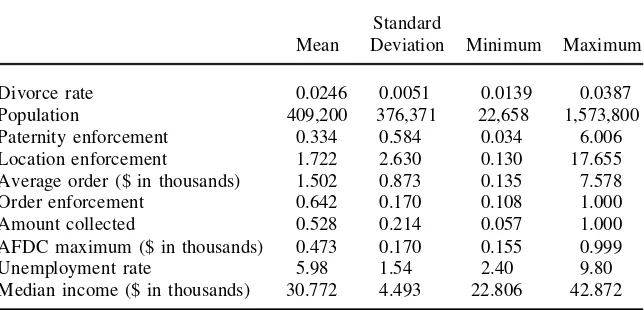
Summary statistics are presented in Table 1. The average state in my sample has an annual divorce rate among married couples with children of 2.46 percent.
B. Estimation Strategy
If state CSE policy has a signicant effect on the probability of a married couple with a child getting a divorce, then the state divorce rate of married couples with children should vary signicantly with the strength of CSE policy. If, on the other hand, there is no effect on the divorce rates of these couples, then the coefcients on all of these policy variables should be small and insignicant.
To test, then, whether state-level divorce rates vary signicantly with Child Sup-port Enforcement policy at the state-level, I run a state-level panel regression. I specify the state-level divorce rate estimation equation as
(1) divorceratest5b01b1CSEst1b2Zst1nst,
Table 1
Summary Statistics
Standard
Mean Deviation Minimum Maximum
Divorce rate 0.0246 0.0051 0.0139 0.0387
Population 409,200 376,371 22,658 1,573,800
Paternity enforcement 0.334 0.584 0.034 6.006
Location enforcement 1.722 2.630 0.130 17.655
Average order ($ in thousands) 1.502 0.873 0.135 7.578
Order enforcement 0.642 0.170 0.108 1.000
Amount collected 0.528 0.214 0.057 1.000
AFDC maximum ($ in thousands) 0.473 0.170 0.155 0.999
Unemployment rate 5.98 1.54 2.40 9.80
Median income ($ in thousands) 30.772 4.493 22.806 42.872
whereCSEstcontains one or more measure of Child Support Enforcement policy,
Zstare demographic or economic characteristics of state s at time t, andnstis the
error term.15A two-stage GLS estimation procedure is used, which accounts for the heteroskedasticity in the error term that results from differential sampling rates of divorce records across states.16
Since a couple’s nancial situation has been found to affect the likelihood of their
15. A log-odds ratio specication was also estimated. The general results remain unchanged when the model is specied in this way.
16. The variance of the error term comes from two sources. The rst is due to sampling variation, or the error in measuring the proportion of divorces that occurred among couples with children under 18, since in many states the Vital Statistics data samples only a subset of all divorce records. The second part is due to lack of t of the model. Thus, the variance of the error term is
(2) s2
Lettingpˆstbe the proportion of sampled divorces occurring to couples with children under 18,nstbe the total number of sampled divorces, anddstbe the total number of divorces in statesin yeart, my estimate of the divorce rate among couples with children under 18 is
(3) divorcˆeratest5
pˆstdst
populationst .
Thus, adapting from Maddala (1983), a consistent estimate of the rst term of the variance is (4) sˆ2
Estimation proceeds following a modication of the procedure outlined in Dickens (1990). First, an un-weighted regression of Equation 1 is performed. Second, the Maddala approximation ofsˆsvst(or 0 if all
records were sampled) is subtracted from the squared residuals of this regression, constraining the results to be greater than or equal to zero, to ensure that total variation is at least that which would come from sampling variation. The mean of these is then taken to yield an estimate ofsˆ2
lof. Third, weights are created, which are the square root of the inverse of the estimatedsˆ2
remaining married,17the state-level unemployment rate and the state-level median money income are included in the regressions. In addition, Ellwood and Bane (1985) nd a signicant negative effect of welfare generosity on divorce rates. To account for this, the maximum AFDC benets for a family of four is also included in the estimation.
Of course, various other factors may affect the divorce rate in a state at a given time, including the religious and ethnic makeup of a state, the legal environment, and underlying attitudes toward divorce, whether within a state or nationwide. Most of these factors are either largely unchanging from year-to-year, or data on these at the state or national level are either not available or poorly measured on a year-to-year basis. To control for these various factors, time and state xed effects are in-cluded in various regressions.
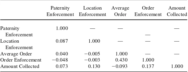
Following Nixon (1997), state-level divorce rates of married couples with children are initially regressed against each of the policy variables in separate regressions with and without the economic variables. However, contrary to Nixon’s data, my measures of CSE policy are not highly correlated (see Table 2), and so I am also able to include them jointly in a regression. Time xed effects are then added to control for unobserved variables that affect the probability of divorce nationally. Finally, state xed effects are included to control for unobserved or slowly changing variables that affect divorce rates, and for differences in attitudes toward divorce across states.
V. Results
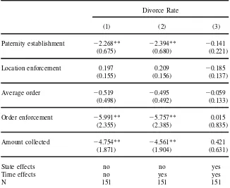
In the rst column of Table 2, I regress the divorce rate separately against each of the measures of child support enforcement policy, with no state or time xed effects included. As such, all sources of variation in divorce rates are used to identify the effects of the Child Support Enforcement variables. In several of these regressions, Child Support Enforcement policy is found to have a signicant negative effect on the prevalence of divorce.
Estimation of the effect of the paternity enforcement variable alone yielded a sta-tistically signicant negative coefcient. This estimate implies that a standard devia-tion increase in the level of paternities established would reduce the divorce rate by 0.128 percentage points, or 5.2 percent. This is somewhat puzzling, because for married couples, paternity of the children would likely not be in doubt, so the pater-nity enforcement effort would not be expected to yield much of an effect. In addition, referring back to Table 2, this variable is not highly correlated with any of the other regressors, so it is unlikely that what I am picking up is the effect of some other policy variable.
Both order enforcement and the amount collected also entered with signicant negative coefcients, implying that a one standard deviation increase in each of these variables would yield decreases in the divorce rate on the order of 4.08 percent and 4.14 percent, respectively.
Location enforcement alone, on the other hand, is estimated to have a positive
Table 2
Correlations Between Child Support Enforcement Policy Variables
Paternity Location Average Order Amount Enforcement Enforcement Order Enforcement Collected
Paternity 1.000 — — —
Enforcement —
Location 0.087 1.000 — — —
Enforcement
Average Order 0.040 20.005 1.000 — — Order Enforcement 20.048 20.003 0.430 1.000
Amount Collected 0.073 0.130 20.093 0.137 1.000
effect on divorce rate. The coefcient of 0.000197 implies that a standard deviation increase in location enforcement efforts would increase divorce rates by 2.11 percent. This coefcient is, however, insignicant. The average order awarded also had an insignicant coefcient, but the coefcient of20.000519 implies that a standard deviation increase in the average order awarded would decrease divorce rates by 1.84 percent.
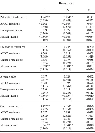
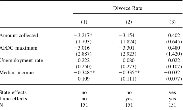
In Column 2 of Table 3, time xed effects are added to the regression, and these same general conclusions are found. In these specications, cross-sectional variation is still being used to identify the coefcients, and since Nixon included time xed effects in that study’s pooled cross-section estimations, these specications use the same type of identifying variation. Scanning this column, the same general conclu-sions noted above are found. Paternity establishment, order enforcement, and the amount collected all have signicant negative coefcients of similar magnitude to those found in regressions that did not include time xed effects, and location en-forcement and the average order both enter insignicantly. Further, in Columns 1 and 2 of Table 4, when economic variables are included in the estimated equations, this pattern of signicance largely remains, though the coefcients are slightly smaller in absolute value.
Thus, when using cross-sectional variation, it appears that at least some measures of CSE policy have signicant effects on the prevalence of divorce, and that these effects tend to be negative.
Table 3
Regressions with Child Support Enforcement Measures Entered Separately
Divorce Rate
(1) (2) (3)
Paternity establishment 22.268** 22.394** 20.141
(0.675) (0.680) (0.221)
Location enforcement 0.197 0.209 20.185
(0.155) (0.156) (0.137)
Average order 20.519 20.495 20.059
(0.498) (0.492) (0.133)
Order enforcement 25.991** 25.757** 0.015
(2.355) (2.385) (0.835)
Amount collected 24.754** 24.561** 0.421
(1.871) (1.904) (0.631)
State effects no no yes
Time effects no yes yes
N 151 151 151
Note: Coefcients reported in table are regression coefcients31023. Each horizontal panel reports the
coefcients from separate regressions, with the independent variables being the CES measure, a constant, and time and/or state xed effects where noted. The dependent variable is the state-level divorce rate in a given year among couples with children under the age of 18. Standard errors are in parentheses. ** Signicant at the 5 percent level.
* Signicant at the 10 percent level.
are included is merely 5.8 percent of the effect when they are not, and the estimated effect of order enforcement is 0.2 percent of its former size.18
These results could, however, explain the puzzling signicant negative coefcient found on the paternity establishment variable, in that it seems plausible that paternity
18. It has been noted, for example, in Altonji and Segal (1996), that when using optimal minimum distance GMM estimators, estimates may be biased downward in absolute value. Since the estimates presented here are of this type, I have rerun these regressions without using any weights to ensure that coefcients are not insigni cant due to a downward bias in the estimators.
Table 4
Regressions with Child Support Enforcement Measures Entered Separately and Economic Variables Included
Divorce Rate
(1) (2) (3)
Paternity establishment 21.867** 21.959** 20.141
(0.639) (0.645) (0.225)
AFDC maximum 22.262 22.643 0.494
(2.850) (2.873) (1.421)
Unemployment rate 0.319 0.176 0.023
(0.243) (0.265) (0.107)
Median income 20.363** 20.344** 20.034
(0.107) (0.108) (0.077)
Location enforcement 0.232 0.242 20.200
(0.154) (0.155) (0.000)
AFDC maximum 24.563 25.015 20.639
(3.093) (3.135) (1.419)
Unemployment rate 0.336 0.179 20.055
(0.255) (0.279) (0.109)
Median income 20.328** 20.309** 20.037
(0.113) (0.115) (0.076)
Average order 0.087 0.123 0.062
(0.477) (0.482) (0.135)
AFDC maximum 23.063 23.392 0.678
(3.111) (3.145) (0.149)
Unemployment rate 0.256 0.115 0.038
(0.261) (0.285) (0.112)
Median income 20.368** 20.357** 20.010
(0.115) (0.116) (0.088)
Order enforcement 24.497** 24.250* 20.076
(2.217) (2.250) (0.866)
AFDC maximum 22.697 22.995 0.429
(2.882) (2.922) (1.421)
Unemployment rate 0.278 0.146 0.018
(0.246) (0.270) (0.107)
Median income 20.361** 20.348** 20.040
Table 4 (continued)
Divorce Rate
(1) (2) (3)
Amount collected 23.217* 23.154 0.402
(1.793) (1.824) (0.645)
AFDC maximum 23.016 23.301 0.480
(2.887) (2.923) (1.420)
Unemployment rate 0.222 0.080 0.022
(0.250) (0.273) (0.107)
Median income 20.348** 20.335** 20.032
0.109 (0.111) (0.077)
State effects no no yes
Time effects no yes yes
N 151 151 151
Note: Coefcients reported in table are regression coefcients31023. Each horizontal panel reports the
coefcients from separate regressions, with the independent variables being the CSE measure, economic variables, a constant, and time and/or xed effects where noted. The dependent variable is the state-level divorce rate in a given year among couples with children under the age of 18. Standard errors are in parentheses.
** Signicant at the 5 percent level * Signicant at the 10 percent level.
establishment effort is highly correlated with other unobservable aspects of a state that tend to discourage divorce, resulting in a spurious negative correlation between the two when cross-sectional variation is used.
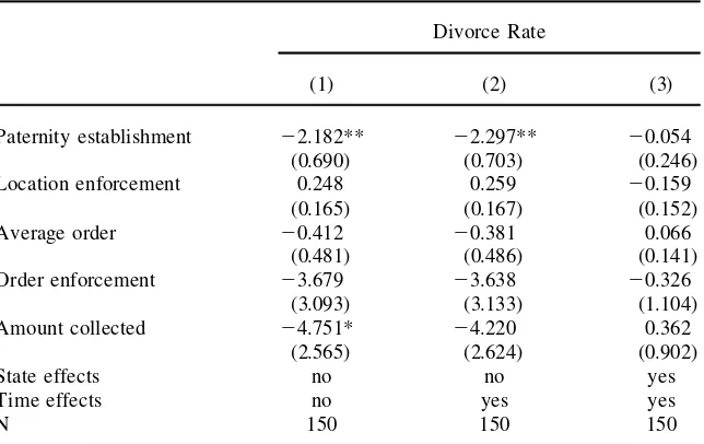
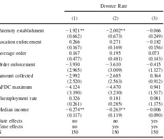
In Tables 5 and 6, all of the child support measures are jointly included in a regression. In this regression, the pattern found above stays roughly the same. When only the CSE measures are included, both the paternity establishment and the amount-collected variables enter signicantly, with negative signs and sizable coef-cients of20.002182 and20.004751, respectively. The order enforcement variable drops to insignicance, but still has a sizable coefcient. Overall, the magnitudes of all coefcients are similar to those from the regressions in which they were entered separately. Further, this pattern of signicance remains when economic variables and time xed effects are included. Again, however, when state xed effects are added, the coefcients drop greatly in magnitude, and all become insignicant.
parame-Table 5
Regressions with all Child Support Enforcement Measures Included
Divorce Rate
(1) (2) (3)
Paternity establishment 22.182** 22.297** 20.054
(0.690) (0.703) (0.246)
Location enforcement 0.248 0.259 20.159
(0.165) (0.167) (0.152)
Average order 20.412 20.381 0.066
(0.481) (0.486) (0.141)
Order enforcement 23.679 23.638 20.326
(3.093) (3.133) (1.104)
Amount collected 24.751* 24.220 0.362
(2.565) (2.624) (0.902)
State effects no no yes
Time effects no yes yes
N 150 150 150
Note: Coefcients reported in table are regression coefcients31023. The independent variables in the
above regressions are the CSE measures, a constant, and time and/or state xed effects where noted. The dependent variable is the state-level divorce rate in a given year among couples with children under the age of 18. Standard errors are in parentheses.
** Signicant at the 5 percent level. * Signicant at the 10 percent level.
ters. However, when state xed effects are added, so that identication comes from within state over time variation, the coefcients drop to essentially zero, and are all insignicant.
To probe this further, I reran all of the regressions using the divorce rate among childless couples as the dependent variable. In these regressions, we would expect there to be no effect of child support enforcement on the divorce rate, since child support payments would not be an issue if the couple were to divorce. These results, presented in Table 7, show a remarkably similar pattern to those reported above. Namely, when cross-sectional variation is used to identify the parameters, paternity enforcement, order enforcement, and the amount collected all enter negatively and signicantly.19However, when state xed effects are included in the regression, the coefcients again drop in magnitude and become insignicant.20Because we would not expect child support enforcement to have any effect on these divorce rates, the signicant negative coefcients when state xed effects are not included in the
re-19. This is in contrast to the robustness checks in Nixon’s paper, where no signicant effect of CSE policy on the divorce behavior of women without children is found.
Table 6
Regressions with all Child Support Enforcement Measures and Economic Variables Included
Divorce Rate
(1) (2) (3)
Paternity establishment 21.921** 22.002** 20.066
(0.662) (0.673) (0.249)
Location enforcement 0.266 0.271 20.182
(0.167) (0.169) (0.156)
Average order 0.167 0.195 0.073
(0.477) (0.481) (0.143)
Order enforcement 23.930 23.610 20.415
(2.965) (3.009) (1.127)
Amount collected 22.992 22.685 0.364
(2.520) (2.563) (0.912)
AFDC maximum 24.124 24.470 0.941
(3.190) (3.230) (1.517)
Unemployment rate 0.326 0.181 0.081
(0.261) (0.285) (1.175)
Median income 20.274** 20.263** 20.006
(0.117) (0.119) (0.090)
State effects no no yes
Time effects no yes yes
N 150 150 150
Note: Coefcients reported in table are regression coefcients31023. The independent variables in the
above regressions are the CSE measures, economic variables, a constant, and time and/or state xed effects when noted. The dependent variable is the state-level divorce rate in a given year among couples with children under the age of 18. Standard errors are in parentheses.
** Signicant at the 5 percent level. * Signicant at the 10 percent level.
gression again suggests that in using cross-sectional variation, the coefcients on the CSE variables might be picking up the effect of unobserved state characteristics that tend to favor stronger CSE policy and frown upon divorce.
VI. Discussion
Table 7
Regressions with Child Support Enforcement Measures Entered Separately: Couples Without Children
Divorce Rate
(1) (2) (3)
Paternity establishment 22.674** 22.766** 20.176
(0.804) (0.819) (0.200)
Location enforcement 0.048 0.055 0.029
(0.185) (0.188) (0.126)
Average order 0.366 0.390 0.121
(0.575) (0.585) (0.809)
Order enforcement 25.813** 25.750** 20.373
(2.822) (2.879) (0.762)
Amount collected 27.775** 27.796** 21.022
(2.186) (2.240) (0.570)
State effects no no yes
Time effects no yes yes
N 151 151 151
Note: Coefcients reported in table are regression coefcients31023. Each horizontal panel reports the
coefcients from separate regressions, with the independent variables being the CSE measure, a constant, and time and/or state xed effects where noted. The dependent variable is the state-level divorce rate in a given year among couples without children. Standard errors are in parentheses.
** Signicant at the 5 percent level. * Signicant at the 10 percent level.
policy on the divorce rate, the estimates yielded from this study show that the effect is extremely small.
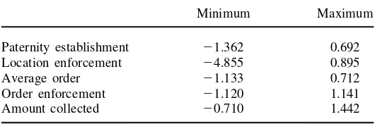
To illustrate this, in Table 8, I calculate the endpoints of the 95 percent condence interval of the effect of a standard deviation increase in each of the child support enforcement measures in Column 3 of Table 3. This column contains roughly repre-sentative effects of the child support enforcement measures when both state and time xed effects are included. These gures make it clear that any effect of child support on the divorce rate, positive or negative, are extremely small. The most negative effect found in any of the 95 percent condence intervals was found for location enforcement, in which a standard deviation increase in location enforcement would decrease the divorce rate by 4.9 percent. The largest positive effect in any condence interval was found for the amount collected, in which a standard deviation increase in the amount collected yields a 1.4 percent increase in the divorce rate. When one considers that the standard deviation of the divorce rate is roughly 20 percent of the average divorce rate, these effects seem quite small.
Table 8
Bounds of the 95 Percent Condence Interval of Effect of Standard Deviation Increase in CSE Variable as Percentage of Average Divorce Rate
Minimum Maximum
Paternity establishment 21.362 0.692
Location enforcement 24.855 0.895
Average order 21.133 0.712
Order enforcement 21.120 1.141
Amount collected 20.710 1.442
is different in the two papers, with ‘‘divorce’’ in the Nixon paper dened as becom-ing separated or divorced in the previous ve years, whereas ‘‘divorce’’ in this paper is dened as becoming divorced in a given year. Hence, the coefcients in the two papers are not directly comparable. Although it seems unlikely, it may be that the greatest effects of Child Support Enforcement are on the decision of whether or not to separate, instead of on the divorce decision.
Further, it should be remembered that these estimates did not include all states over the years of analysis. Data were only available from states that collected and assembled Vital Statistics data from their divorce records, and this had the effect of excluding nearly 20 states each year from the analysis. It may be that the effect of CSE on divorce was most signicant in those states for which I do not have data, and had those states been included, the results may have been different.
Finally, this study covers only a ve year time span, 1991– 95, due to data con-straints.21Although some variation exists across states and time in the measures of child support enforcement effectiveness, a substantial part of the increase in child support enforcement had already passed by the beginning of the time period ana-lyzed. Since Nixon’s data come from 1988 and 1990, it may be that divorce rates were more reactive to Child Support Enforcement policy in earlier years. While it would have been advantageous to include more years of data, this data is simply not available for the measures that were used in the present study.
Notwithstanding the above, the change in signicance and large drop in the magni-tude of coefcients when state xed effects strongly argues against using only cross-sectional variation in order to identify the effects of child support enforcement on divorce.
VII. Conclusion
This paper attempted to measure how much, and in what direction, the changes in child support enforcement policy during the Bush and Clinton
istrations had on the divorce rate of couples with children. These estimates show that some measures of Child Support Enforcement policy had a signicant negative effect when only cross-sectional variation was used, but that these became much smaller and insignicant once state xed effects were included.
Thus, it appears that, regardless of what effect the changes in Child Support En-forcement policy had on the receipt of child support by single parents, these changes did not erode or enforce marital stability.
A number of explanations may be offered. For example, informational consider-ations may need to be taken into account. It may be that people simply did not know about the changes in Child Support Enforcement, or could not infer the magnitude of the changes, and hence could not alter their behavior accordingly. More likely, however, is that the decision to divorce may be such a complex decision, with so many factors playing into it, that variables like the strength of child support enforce-ment policy play an extremely minimal role.
Therefore, when examining issues surrounding the Child Support Enforcement effort in the United States, it is likely much more worthwhile to consider the direct effects of this program, such as the probability of receipt of support for the custodial parent, or outcomes of the children who receive child support. These results suggest that its effects on divorce, whether positive or negative, are minimal.
References
Altonji, Joseph G., and Lewis M. Segal. 1996. ‘‘Small Sample Bias in GMM Estimation of Covariance Structures.’ ’Journal of Business and Economic Statistics 14(3):353– 66.
Bloom, David E., Cecilia Conrad, and Cynthia Miller. 1998. ‘‘Child Support and Fathers’ Remarriage and Fertility.’’ InFathers Under Fire: The Revolution in Child Support En-forcement, ed. Irwin Garnkel et al, 128–56. New York: Russell Sage Foundation. Committee on Ways and Means, U.S. House of Representatives. (Various).Green Book.
Washington, D.C.: GPO.
Dickens, William T. 1990. ‘‘Error Components in Grouped Data: Is It Ever Worth Weighting?’’Review of Economics and Statistics 72(2):328– 33.
Ellwood, David T., and Mary J. Bane. 1985. ‘‘The Impact of AFDC on Family Structure and Living Arrangements.’ ’ InResearch in Labor Economics. Vol. 7. ed. Ronald Ehren-berg, 137–207. Greenwich, Conn.: JAI Press.
Freeman, R., and J. Waldfogel. 2001. ‘‘Dunning Delinquent Dads: The Effects of Child Support Enforcement Policy on Child Support Receipt by Never Married Women.’’ Jour-nal of Human Resources36(2):207– 25.
Friedberg, Leora. 1998. ‘‘Did Unilateral Divorce Raise Divorce Rates? Evidence from Panel Data.’’American Economic Review88(3):608– 27.
Johnson, William, and Jonathan Skinner. 1986. ‘‘Labor Supply and Marital Separation.’’
American Economic Review76(3):455– 69.
Maddala, G. S. 1983.Limited-Dependent and Qualitative Variables in Econometrics. New York: Cambridge University Press.
Nixon, Lucia. 1997. ‘‘The Effect of Child Support Enforcement on Marital Dissolution.’’
Journal of Human Resources32(1):159– 81.
———. 1993. ‘‘The Importance of Financial Considerations in Divorce Decisions.’ ’ Eco-nomic Inquiry31:71– 86.
Robins, Philip. 1986. ‘‘Child Support, Welfare Dependency, and Poverty.’’American Eco-nomic Review 76(4):768– 88.
Sweezy, Kate, and Jill Tiefenthaler. 1996. ‘‘Do State-Level Variables Affect Divorce Rates?’’Review of Social Economy 54(1):47– 65.
U.S. Bureau of the Census. 1990. General Population Characteristics. Washington, D.C., U.S. Bureau of the Census.
U.S. Bureau of the Census. 1995. Population Prole of the United States 1995. Washing-ton, D.C., U.S. Bureau of the Census.
U.S. Department of Health and Human Services. 1998. ‘‘Child Support Enforcement: A Clinton Administration Priority.’’ HHS Fact Sheet, June 24, 1998.
U.S. Dept. of Health and Human Services, Administration for Children and Families, Of-ce of Child Support Enforcement. Various.Child Support Enforcement: Annual Report to the Congress. Washington, D.C., U.S. Dept. of Health and Human Services. Yun, Kwi Ryung. 1992. ‘‘Effects of Child Support on Remarriage of Single Mothers.’’ In