T H E J O U R N A L O F H U M A N R E S O U R C E S • 46 • 4
William R. Johnson
A B S T R A C T
Hours constraints are typically identified by worker responses to questions asking whether they would prefer a job with more hours and more pay or fewer hours and less pay. Because jobs with different hours but the same rate of pay may be infeasible when there are fixed costs of employment or mandatory overtime premia, the constraint in those cases may be illusory. Cross-section estimates of reported hours constraints are consistent with this model implying that the overall level of hours constraints may exag-gerate the extent to which the labor market is characterized by frictions and imperfections.
I. Introduction
The standard neoclassical theory of labor supply assumes that a worker can choose his preferred hours of work at a constant rate of pay per hour either directly by choosing his hourswithin a job or indirectly by choosing a job that requires the preferred hours. The usual response to the observation that most jobs do not allow much choice of hours is to argue that even if jobs allow no choice of hours, workers can in effect choose their hours by choosing their jobs. In this market equilibrium, every worker will be working as much as he wants even though not every job allows the worker to choose his hours. However, about a third of all U.S. workers say they would like to work either more hours or fewer hours than they currently work at the same hourly rate of pay, an observation that appears to be inconsistent with a frictionless labor market.
There are three distinct reasons a worker might claim to prefer another job with more or fewer working hours than his current job. Most obviously, that preferred job may exist but search frictions keep the worker from finding it costlessly. Thin labor markets would be one reason; the ideal job may exist in large dense labor
William R. Johnson is professor of economics at the University of Virginia. He appreciates helpful com-ments on earlier versions from Leora Friedberg, Helen Levy, Derek Neal, Steve Stern, Sarah Turner, and Jim Ziliak and workshop participants at the University of Virginia, Princeton University, and Dartmouth College. This research was supported by the Bankard Fund at the University of Virginia. The data used in this article can be obtained beginning May 2012 through April 2015 from William Johnson, P.O. Box 400182, Charlottesville, VA 22904 wjohnson@virginia.edu.
[Submitted June 2010; accepted November 2010]
markets with many employers but the worker in a small labor market cannot find the perfect match at the small number of employers nearby.1A second possibility
is that the job is not offered even though it is both feasible and preferred by the worker, implying that employers are leaving potential gains on the table. Finally, the worker’s preferred job may not be offered by employers because in competitive markets it is not feasible; that is, an employer who offered this job would not cover costs. Although hours constraints can arise in noncompetitive markets if the preferred job is not rent-maximizing for a monopsony employer to offer or for a monopoly union to allow, the results in this paper focus on the competitive case and conclude that some hours constraints arise because the preferred job is not feasible. This finding sheds light on the importance of labor market frictions in explaining labor market behavior; hours constraints can exist even in frictionless markets with max-imizing agents.
Data on self-reported hours constraints in this and other studies come from an-swers workers give to questions about whether they would prefer more hours of work earning more money, fewer hours earning less money, or their current hours and earnings. These questions are usually interpreted as implying a choice of hours at the same average hourly earnings, a condition intended to ensure that the worker considers only alternative jobs that are economically feasible.2A worker who prefers
alternative hours is often deemed to face an hours constraint arising from market frictions or imperfections that have kept the worker from a job which he prefers and is economically feasible. Alternative jobs with fewer hours are feasible as long as the worker’s marginal contribution to output is no greater than the worker’s marginal cost to the employer, a situation which holds if (but not only if) both output and labor cost are strictly proportional to hours worked as they are when labor costs are only a constant hourly wage and hourly labor productivity is constant. However, worker output is not proportional to hours when there are setup costs or fatigue effects (Hamermesh 1993). Likewise, labor costs are not proportional to hours under mandatory overtime premia (Ehrenberg 1971) or fixed-cost fringe benefits. In these cases, alternative jobs at the same hourly rate of pay may not be feasible so the fact that a worker would prefer them does not indicate a real hours constraint. The constraint is illusory.
To motivate the empirical work, the paper sketches a model with search frictions along with two reasons for marginal productivity not to equal marginal labor cost— fixed cost fringe benefits and overtime premia. Fatigue effects or setup costs are not easily observed, but fixed-cost fringe benefits are, so the paper focuses on them. The model makes two strong empirical predictions. First, it predicts that, compared to equally productive workers in jobs without fringes, workers in jobs with fringe benefits whose cost is not proportional to hours worked (fixed-cost fringe benefits)
1. Complementarities between worker hours at the same employer might lead employers to require uniform hours within a firm or establishment. If the number of firms in a labor market is small, workers may not be able to find an employer offering jobs with their preferred hours. This suggests that more workers would report being constrained in small labor markets than big ones with more choice. In the data, however, the opposite is true.
will be more likely to want to work less and less likely to want to work more,even holding constant their actual number of hours. Second, it predicts that when com-paring a worker’s hours at two points in time, workers who initially want to work more will increase their hours, workers who want to work less will decrease their hours, but the effect of wanting to work less on subsequent hours reductions will be much smaller for workers with fixed-cost fringe benefits. Both of these predictions are strongly confirmed by data on self-reported hours constraints from the Current Population Survey (CPS).
To understand clearly and simply the nature of the empirical results in the paper, consider two workers with identical and constant hourly productivity, v. In a fric-tionless labor market these two workers can choose among jobs with any combi-nation of fixed-cost fringe benefits,F, weekly hours,h, and hourly wage,w, such that total compensation, FⳭwh, equals the worker’s output, vh. Employers don’t care about the composition of total compensation as long as their labor costs don’t exceed worker output, and competition among employers for workers drives com-pensation to equal output. So in equilibrium, viable jobs satisfy (vⳮw)h⳱F.
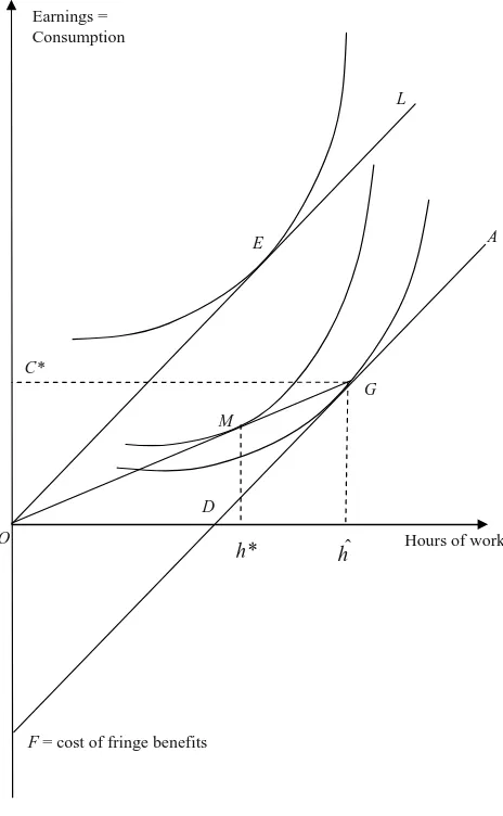
Imagine that these two workers with identicalvdiffer in their preferences forF. One worker has no desire forF, and so chooses a job with noF. By the equilibrium condition, this worker’s wage rate will equalvindependent of the hours of the job. In Figure 1, lineOL with slopevrepresents all feasible jobs with F⳱0 andw⳱v. This worker chooses his most preferred of these jobs, in this case represented by point E. The second worker values F, and so chooses a job with amount of F
represented by the distanceOF. The feasible combinations of hours,h, and earnings,
wh, for this worker are given by line FDA, also with slope v but with vertical intercept,ⳮF. This worker chooses the job at pointGwith hours . The (average)ˆh wage rate at this job is average hourly earnings or w⳱vⳮF/hˆ, the slope of line
OG.
Now suppose both of these workers are asked if they would prefer to work more or less at the same wage rate. The first worker, whose current job is pointEwith a wage rate equal tov, the slope of lineOL, naturally compares other points on the lineOLwith his current job at pointEand answers that he has no desire to change hours. The second worker assumes that the question is asking about jobs with dif-ferent hours at his current wage rate and the same amount of fringe benefits as he currently gets, since fringe benefits are not mentioned in the question. Those jobs would fall along lineOGand its extension since the slope ofOGis his current wage rate. This second worker will answer that he prefers the job atMwith fewer hours, . Thus the first empirical prediction is that comparing workers with identical
* ˆ
h h
hourly productivity,v, workers with more fixed cost fringe benefits,F, will be more likely to say they would like to work fewer hours than they currently work. This is essentially what is shown in Tables 3–5, where we control for v with observable characteristics of worker and jobs.
h*
A E
D
G C*
M
ˆ
h
F = cost of fringe benefits
Earnings = Consumption
L
Hours of work
O
Figure 1
Fringe Benefits and Hours Constraints
instead taken a job atL with more hours than his ideal job atE. That worker will want to search in hopes of finding a job closer to his ideal job atE, a job that would necessarily entail fewer hours.
preferred point on that line. He would prefer to be at point Mon lineOGbut the jobs on lineOGare not feasible. When he is asked whether he would like to work more or fewer hours at the same rate of pay, he is invited to imagine that he can find a job likeMand may search for one but he will not be successful. In this sense, his hours constraint is illusory; he is already at his most preferred feasible job.
If we observe these two workers a period of time after asking whether they would like to work less, the second worker may well have succeeded in reducing his hours but the first worker will not be successful in reducing his hours. Hence workers with fixed cost fringe benefits (like the first worker) who say they would like to work less will be less successful (or not successful at all) in reducing their hours. This is the basic finding in Table 6.
II. Background
Employers typically do not give workers much discretion to choose hours of work; instead, employers offer “jobs” that are tied packages of earnings, hours, and fringe benefits, which can either be accepted or rejected. Of course, workers can choose among jobs and in that way choose hours,3so the fact that some
workers say they would like to work more or less is still a puzzle to explain. Why don’t workers find jobs which match their preferences?
For the most part, the existing empirical literature on hours constraints in labor supply focuses not on the causes of these constraints but on issues such as the effect of hours constraints on labor supply estimates (Ham 1982, Kahn and Lang 1991) and the extent to which hours are constrained (Dickens and Lundberg 1993, Stewart and Swaffield 1997). Altonji and Paxson (1988, 1992) show that workers seek to bring their actual hours closer to their preferred hours when they change jobs. Bloe-men (2008) builds a model in which workers search along two diBloe-mensions, wages and required hours, but the distribution of jobs and their hours requirements is taken as exogenous in his model. Cutler and Madrian (1998) point to evidence that rising health insurance costs have led to increased hours of work per worker as employers seek to cover increased fixed costs of employment. However, their empirical study does not directly observe evidence on hours constraints but only hours of work. Biddle and Zarkin (1989) and Aaronson and French (2004), among others, provide substantial evidence that wage rates depend positively on hours of work, as fixed costs of employment imply. Rogerson and Wallenius (2009) show the importance of this assumption for macroeconomic models of labor supply.
A series of papers by Kahn and Lang (1992, 1995, 1996) test alternative models of hours constraints. Their 1996 paper notes that hours constraints arise when what they call the marginal wage (really a productivity measure, like v in our model) differs from the average wage, or average hourly earnings (vⳮF/hˆ). Workers choose labor supply by equating the marginal value of leisure to the marginal wage. If asked about working any number of hours at the average wage of their current job, they would choose more hours if the average wage exceeds the marginal wage and would
choose fewer hours if the average wage is less than the marginal wage. Kahn and Lang find that the pattern of reported hours constraints is consistent with the shape of the wage-hours locus they estimate at least under certain specifications, but, as they note, it is difficult to identify a locus of wages and hours available to a single worker from data on hours and earnings across workers. They do not use information on fringe benefits or other fixed costs. In later work, Lang and Kahn (2001) conclude that hours constraints are best explained by a “matching model in which wages depend on hours as in hedonic models, but in which the matching is imperfect.”
Like Kahn and Lang, this paper focuses on situations in which earnings are not proportional to hours in the context of costly worker search. The paper brings two new elements to bear on the analysis. First, I use observable determinants of the wage-hours locus, namely fringe benefits, to explain why some workers are more likely to report being constrained. In particular, I show both theoretically and em-pirically that comparing equally productive workers with the same actual hours, those with fringe benefits are more likely to report wanting to work less. Second, I follow workers over time and show that while constrained workers tend to find better matches over time, as a matching model would predict, constrained workers with fringe benefits are less likely to do so, because their current jobs are more likely to be the most preferred feasible jobs. In that sense, the hours constraints they report are “illusory.”
In the data I use, more workers report wanting to work more than report wanting to work less.4 However, the novel results of the paper involve those who want to
work less because fringe benefits imply that hourly productivity exceeds average hourly earnings, so workers want to work less at their average wage. I do include one explanation for wanting to work more (a proxy for overtime premia) but ex-plaining why some workers want more hours is not the central focus of this paper.
III. Hours Constraints
A. Theory
This section describes a simple model of hours constraints to motivate the empirical work which seeks to explain why some workers report hours constraints. Attention is focused on search frictions and the divergence between marginal hourly produc-tivity and marginal labor cost caused by fixed-cost fringe benefits and by legally mandated overtime wage premia. I do not include two additional causes of con-straints, market power or implicit contracts. Monopsony power of employers or monopoly power of labor unions might lead to hours constraints as the agent with market power will not be indifferent about total hours of labor at a given wage rate. Monopsonists can do better if they can push workers off their labor supply curves and monopoly unions will want to curb their members’ desire to work more at the
union wage.5Implicit contract models are alternatives to continuously clearing spot
labor markets, breaking the link between the current wage and hours of work. In risk-sharing implicit contract models, hours are determined efficiently by equating the value of marginal product with the marginal opportunity cost of labor, but wages are determined by long-run risk-sharing criteria. Hence, as the value of marginal product varies over the business cycle, the contract, which is efficient in the long run, will require workers to work hours they would not choose to work at the wage they are paid (Beaudry and di Nardo 1995, Ham and Reilly 2002). Kahn and Lang (1992) reject the implicit contract explanation empirically.
Suppose firms compete for equally productive workers in a competitive labor market by offering jobs which can be characterized as a vector of monetary com-pensation or consumption (C), weekly hours ( ), and weekly fringe benefits (ˆh F). To motivate why firms rather than workers are buying the fringes, one can invoke tax considerations or adverse selection in the insurance market. For our purposes, we simply stipulate that only firms can buy fringe benefits. Each hour of the worker’s labor is assumed to be worth vto each firm so marginal product is independent of hours worked.
A firm that offers jobj,(Cj,hˆj,Fj), and successfully employs a worker at that job, will earn profits,j, where
ˆ
⳱v•hⳮFⳮC
(1) j j j j
The profit a firm earns from hiring a worker is just the difference between the worker’s value of output, v•hˆj, and the wage and fringe cost of employing him. Workers evaluate jobs according to their preferences for consumption, leisure (non-work time) and the fringe benefit. Equilibrium in the labor market is characterized by an assignment of workers to jobs, a zero-profit condition for firms, and, for workers, the existence of no superior job choice. This is a pure compensating dif-ferential equilibrium. By the zero-profit condition for firms, jobs with many fringe benefits must have either lower monetary compensation per hour or greater required hours. The problem is formally equivalent to workers selectingFandhto maximize their utility subject to the constraint that the value of output produced by the worker equals the cost of fringes and earnings.
In equilibrium, therefore, if workers can costlessly search among jobs, each jobj
observed must be the solution to some workeri’s maximization problem:
i
max U(v•hⳮF,Tⳮh,F)
(2) j j j j
F,h
{ j j}
HereTrepresents total time to be allocated between leisure and work. The pattern of jobs observed in the market will, of course, depend on the pattern of preferences for fringe benefits and leisure among workers.
To illustrate, suppose workeri’s utility is log linear in consumption, leisure, and fringes: where 0ai1, 0ⱕbi1. The two preference
ai 1ⳮai bi (v hi ⳮF) •(Tⳮh) •F ,
parameters are ai, the relative weight on consumption in the consumption-leisure subutility function, and bi, the weight on fringes,. The optimal choices ofhandF
are
冢
aiⳭbi冣
T and冢 冣
bi v Ti , respectively. With those choices, a worker’s con-1Ⳮbi 1Ⳮbisumption will be
冢 冣
ai v Ti . Average hourly earnings is consumption divided by 1Ⳮbihours, or a vi i . The job chosen by a worker with preference parameters (aiⳭbi)
and productivityviwill therefore be characterized by: ai andbi
Now suppose the worker who works at his most preferred feasible job as char-acterized by (3) is asked whether he would like to work more or less at the same rate of pay. It is reasonable to think that in answering this question the worker envisions alternative jobs with the same fringe benefits,Fi, but a choice of hours
implying consumption equal to hours times his current average hourly earnings. In Figure 1, the worker at pointGenvisions job possibilities along segmentOG, where the slope ofOGis his current average hourly earnings. Using our specific functional form, the worker envisions the following problem:
ai
Here the only choice variable ishand consumption is thought by the worker to be average hourly earnings, a vi i/(aiⳭbi), times hours. Fringes are fixed at Fi. The solution to this problem is desired hoursh*⳱a T. As long as fringes are positive
i i
(bi0), the jobs alongOGare not feasible because the firm makes negative profits in that region. Hence the job alongOGwith the consumption and hours the worker would like cannot be offered by employers.
The gap between actual and desired hours, ˆhⳮh*, is given by:
i i
hours constraints. Graphically, lineFAand lineOGcoincide. As Equation 5 shows, hours constraints depend on the utility weight on leisure,1ⳮa and the difference
between the slopes ofOGandFA, which depends onFiand in turnbi, the preference weight on fringes.
To express the gap between actual and desired hours as a function of observables, substitute forFi
*
ˆhⳮh ⳱(1ⳮa)(F/v)
(6) i i i i i
This suggests that cross section variation in hours constraints will be a positive function of observed fringes and a negative function of hourly productivity, with additional variation introduced by the preference term1ⳮa.
i
B. Search Frictions
Now consider search frictions. Bloemen (2008) shows that when workers care about both wage rates and required hours, their optimal search strategy is to set a reser-vation utility level and accept any job which meets it. For simplicity, I assume that the frictions result in workers accepting jobs with their desired fringes but with required hours on the job that may vary from their preferences. All jobs are still assumed to generate zero profits for firms. Let εij denote the noise in hours for workeriat jobj:
aiⳭbi
ˆh ⳱ TⳭε
(7) ij
冢
冣
ij1Ⳮbi
Because fringe benefits are at their desired value
冢 冣
bi v Ti , and jobs follow the 1Ⳮbizero profit constraint, consumption equals ai v TⳭε v.
i ij i
冢 冣
1Ⳮbi
If we now rerun the thought experiment of asking the worker whether he would like to work more or less at the same rate of pay, we again assume that the worker assumes that fringe benefits are held constant and desired hours are againh*⳱a T.
i
The gap between actual and desired hours is now
bi *
ˆh ⳮh ⳱ (1ⳮa)TⳭε
(8) ij i
冢 冣
i ij1Ⳮbi
The noise is just added to the previous gap. Writing the gap as a function of ob-servables, we have
implying that the gap is increasing in fringes and actual hours, ˆhij, decreasing in worker productivity,vi, with additional variation implied by differences in the taste
parameters,aiandbi. We can attempt to control for differences in productivity and
tastes with other observables, but this equation predicts that workers who choose jobs with more fringe benefits will report a greater gap between actual and desired wages, even holding constant their actual hours, . As Equation 9 is written, allowingˆh
across workers and will be correlated with the unobservable term
冢 冣
aⳭb T. How-1Ⳮbever, if we restrict the variation in tastes across workers to variation only in the utility weight on fringes, b, holdinga constant, the coefficient on F/vwill be the
same for each worker and the additive unobservable term
冢 冣
aⳭb Twill capture all 1Ⳮbthe taste variation.
C. Overtime Premia
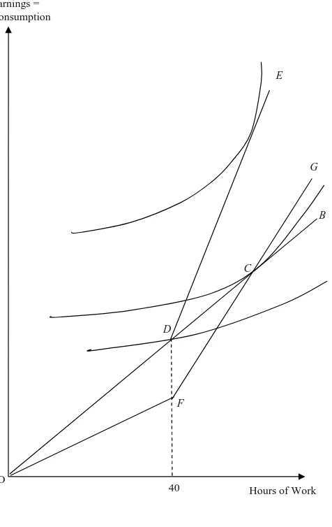
Legally mandated overtime premia also can give rise to hours constraints. To illus-trate simply, assume that fringes are zero and that worker value to the firm is again a constantvper hour so that the competitive wage, before the imposition of overtime premia, equalsv. Firms have no interest in constraining hours. When an overtime premium is imposed on weekly hours above 40, a naı¨ve approach assumes that the straight-time wage continues to equalv. Now firms will constrain hours to be fewer than 40, to avoid paying more for hours than they are worth to the firm. (Ehrenberg 1971). Figure 2 shows the set of feasible jobs as the lineODBwith slopev. In the absence of an overtime premium, a worker chooses point Cand works more than 40 hours. With an overtime premium and the naı¨ve assumption that the straight-time wage stays atv, the constraint becomesODE. Firms will constrain workers to jobs likeDwith 40 hours, when workers would preferC. Note that this explanation does not require the worker to interpret a question about working more as implying that the overtime premium will be paid to him. The firm does not offer C because it cannot legally do so.
Trejo (1991) pointed out that assuming that the straight-time wage remains con-stant with an overtime premium is naı¨ve; the firm could still offer the job initially chosen by the worker at pointC by a suitable adjustment of the straight-time wage rate. OFG represents a straight-time wage and overtime premium that allows the firm to offer job C, which the worker clearly prefers to the naı¨ve constrained job,
D. But at C, the worker may still feel constrained; he would like to work more hours at the overtime rate alongCG. The firm won’t offer a job onCGbecause any job aboveODB is not economically feasible. Again, the hours constraint is caused by the difference between the jobs that are feasible (ODB) and the worker’s per-ceived constraint (OFG). Under either the naı¨ve model or Trejo’s model, workers covered by mandatory overtime premia should be more likely to report wanting to work more.
D. Changes in Hours
Earnings = Consumption
Hours of Work O
D
E
B
C
F
40
G
Figure 2
Overtime Premium
One empirically testable implication is that the effect of wanting to work less on subsequent reductions in hours will be much less (ideally zero) for workers with fixed-cost fringe benefits than for workers without fringes. Preferred jobs with re-duced hours are feasible for the latter group, as illustrated by the worker who because of search frictions lands in jobLin Figure 1 who would prefer job E.
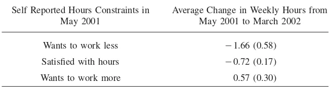
Table 1
Dissatisfaction with Current Hours and Subsequent Changes in Hours
Self Reported Hours Constraints in May 2001
Average Change in Weekly Hours from May 2001 to March 2002
Wants to work less ⳮ1.66 (0.58)
Satisfied with hours ⳮ0.72 (0.17)
Wants to work more 0.57 (0.30)
Source: Matched observations from the CPS in May 2001 and in March 2002 who were employed in both surveys; standard errors in parentheses
jobs without fringe benefits, because hourly earnings cannot be negative or less than the legal minimum wage when that applies.6 Hence, workers initially in jobs with
fringes will work more hours on average and will thus be more likely to reduce hours over time than workers initially in jobs without fringes. By a similar argument, workers in jobs with fringes at the end of the period will be more likely to have increased their hours during the period.
IV. Empirical Tests
A. Data and Descriptive Statistics
Testing this model requires data on hours constraints. The May 2001 Current Popu-lation Survey asked working respondents whether they would prefer to work more for more pay or work less for less pay. The answers to that question form the basis for the empirical work here. Because all the empirical work depends on this self-reported constraint variable, it is worth making sure that survey responses are con-sistent with worker behavior. Table 1 confirms that those workers who said they wanted to work less were, in fact, observed, on average, subsequently reducing their hours, while those workers who said they wanted to work more were later observed increasing their hours on average.
To explore the empirical implications of the model, we need measures of fringe benefits. The CPS asks workers whether the employer contributes to employee health insurance and whether the worker is covered by a pension plan on his job. The CPS then makes an imputation of the amount of the employer contribution to health insurance based on other information like the worker’s industry. Because fringe benefit information is gathered only in the March CPS survey, to combine it with the hours constraint data from May requires merging and matching the participants
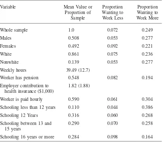
Table 2
Descriptive Statistics
Variable Mean Value or
Proportion of Sample
Proportion Wanting to Work Less
Proportion Wanting to Work More
Whole sample 1.0 0.072 0.249
Males 0.508 0.053 0.277
Females 0.492 0.092 0.221
White 0.861 0.075 0.236
Nonwhite 0.139 0.053 0.277
Weekly hours 39.49 (12.7)
Worker has pension 0.548 0.082 0.194
Employer contribution to health insurance ($1,000)
1.82 (1.88)
Worker is paid hourly 0.590 0.061 0.304
Schooling less than 12 years 0.110 0.044 0.386
Schooling 12 Years 0.316 0.060 0.268
Schooling between 13 and 15 years
0.290 0.070 0.258
Schooling 16 years or more 0.284 0.098 0.164
Note: Matched CPS March 2001 and May 2001 samples. Restricted to individuals employed at same job in both months. Sample mean with sample standard deviation in parentheses.
in the March and May 2001 surveys. Overtime premia are proxied by whether the worker is paid on an hourly basis since he is much more likely to be covered by mandatory overtime premia if he is paid hourly.7
The 2001 matched CPS sample is described in Table 2. About a quarter of all workers say they would like to work more at the same wage while about 7 percent say they would like to work less, for an overall dissatisfaction rate of about a third.8
Males are more likely to want to work more than females are; females are more likely to want to work less. Whites are more likely to want to work less than
7. Workers who are “exempt” from the overtime provisions of federal labor law (FLSA) must be salaried and must perform certain types of duties. It is difficult to determine exactly who is exempt in the CPS, but it is known that hourly employees cannot be exempt.
nonwhites, as are those with high levels of schooling and those who are not paid hourly.
The fact that Table 2 reveals many more workers who want to work more hours than workers who want to work fewer hours may appear to be inconsistent with a model which attempts to explain why workers would say they want to work less. Although the focus of the paper is on the fringe-benefit-illusion story, the empirical work allows for additional causes of hours constraints such as search frictions and overtime premia. Data consistent with the fringe benefit-illusion story do not imply that other explanations of hours constraints are not valid or that they may well explain a greater incidence of hours constraints than the fringe-benefit illusion hy-pothesis. These are complementary explanations not substitutes.
B. Effects of Job and Worker Characteristics on Hours Constraints
This section reports probit estimates of the effect of job and worker characteristics on self-reported hours constraints. All employed workers, whether they are paid hourly or not are included in the main estimates reported in Tables 3–6; parallel estimates for hourly-paid workers only are reported in Appendix Tables A1–A4. The parametric model implies that the gap between actual and desired hours depends positively onF/v. Direct observation ofvis not possible so we cannot test whether the ratio specificationF/vis consistent with the data.9Instead we control forvwith
worker and job characteristics.
Randomness in the empirical model arises from unobserved taste and productivity differences across individuals. It also could arise from variation in individual-specific reporting threshold values. Suppose that a worker reports wanting to work less if the difference between actual hours and desired hours (ˆhⳮh*) exceeds some thresh-old,; if the discrepancy is less than it is too small to report. The values ofin the sample are assumed to be drawn from a normal probability distribution function . The probability that a randomly chosen member of the sample reports working
F()
too much is then Pr(hˆⳮh* ˆ *. Hence with our proxies for the )⳱1ⳮF(hⳮh )
theoretical determinants of the divergence between actual and desired hours, we can test the implications of the alternative hypotheses with a standard probit model.
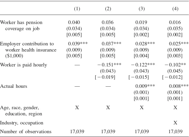
Table 3 reports probits on wanting to work less. Column 1 looks at pension coverage and health insurance. Health insurance, which is more likely than pension coverage to be a true fixed-cost fringe benefit independent of hours worked, is strongly positively related to wanting work less. The effect of pension coverage is also positive, but is not significant. Controls for worker characteristics are intended to capture some of the variation in worker productivity (v) and the preference term
in Equation 9.
aⳭb T
冢 冣
1ⳭbColumn 2 of Table 3 adds a dummy for being paid hourly (and hence eligible for a mandatory overtime wage premium), which is significantly negatively related to wanting to work less, as theory predicts. Column 3 adds the worker’s actual hours
Table 3
Probit Estimates of Hours Constraints: Worker Wants to Work Less
(1) (2) (3) (4)
Worker has pension coverage on job
0.040 0.036 0.019 0.016
(0.034) (0.034) (0.034) (0.035) [0.005] [0.005] [0.002] [0.002]
Employer contribution to worker health insurance ($1,000)
0.039*** 0.037*** 0.028*** 0.025*** (0.009) (0.009) (0.009) (0.009) [0.005] [0.005] [0.004] [0.003]
Worker is paid hourly — ⳮ0.151*** ⳮ0.122*** ⳮ0.102** (0.043) (0.043) (0.045) [ⳮ0.019] [ⳮ0.015] [ⳮ0.012]
Actual hours — — 0.009*** 0.008***
(0.001) (0.001) [0.001] [0.001]
Age, race, gender, education, region
X X X X
Industry, occupation X
Number of observations 17,039 17,039 17,039 17,039
Note: Matched observations from March 2001 and May 2001 Current Population Surveys. Robust standard errors in parentheses. In square brackets are effects of one unit change in variable on probability of wanting fewer hours, evaluated at the means. Each regression includes age, a dummy for white, a gender dummy, three education dummies, eight Census region dummies, and a dummy for missing data on whether worker is paid hourly. (4) adds 13 occupation dummies and 22 industry dummies. *** 0.01 significance, ** 0.05 significance, * 0.10 significance.
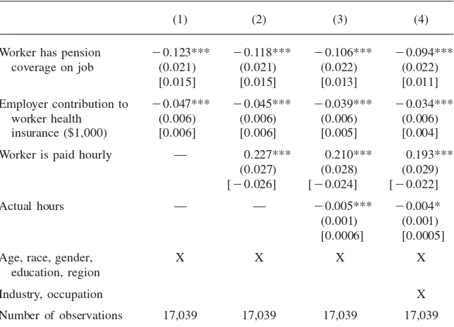
Table 4
Probit Estimates of Hours Constraints: Worker Wants to Work More
(1) (2) (3) (4)
Worker has pension coverage on job
ⳮ0.153*** ⳮ0.148*** ⳮ0.141*** ⳮ0.125*** (0.025) (0.024) (0.025) (0.026) [ⳮ0.047] [ⳮ0.045] [ⳮ0.043] [ⳮ0.038]
Employer contribution to worker health insurance ($1,000)
ⳮ0.051*** ⳮ0.049*** ⳮ0.046*** ⳮ0.039*** (0.007) (0.007) (0.007) (0.007) [ⳮ0.015] [ⳮ0.015] [ⳮ0.014] [ⳮ0.012]
Worker is paid hourly — 0.269*** 0.259*** 0.242*** (0.033) (0.033) (0.034) [0.085] [0.082] [0.076]
Actual hours — — ⳮ0.003*** ⳮ0.002*
(0.001) (0.001) [ⳮ0.001] [ⳮ0.001]
Age, race, gender, education, region
X X X X
Industry, occupation X
Number of observations 17,039 17,039 17,039 17,039
Note: Same as Table 3.
Table 4 reports similar probits on wanting to work more. Here, both types of fringe benefits, pension coverage and health insurance, have significantly negative effects as theory predicts. Pensions as well as health insurance are strongly related to hours constraints. Compared with a worker with no fringes, a worker with pension coverage is roughly four percentage points less likely to report wanting to work more, as is a worker with the mean value of health insurance. These effects are each one-sixth of the mean likelihood of wanting to work more. Being paid hourly raises the probability of wanting to work more by more than one-third of its mean value. And, as in Table 3, these results hold up even when I add actual hours (Column 3) and industry and occupation dummies (Column 4).
Table 5
Ordered Probit Estimates of Hours Constraints
(1) (2) (3) (4)
Worker has pension coverage on job
ⳮ0.123*** ⳮ0.118*** ⳮ0.106*** ⳮ0.094*** (0.021) (0.021) (0.022) (0.022) [0.015] [0.015] [0.013] [0.011]
Employer contribution to worker health insurance ($1,000)
ⳮ0.047*** ⳮ0.045*** ⳮ0.039*** ⳮ0.034*** (0.006) (0.006) (0.006) (0.006) [0.006] [0.006] [0.005] [0.004]
Worker is paid hourly — 0.227*** 0.210*** 0.193*** (0.027) (0.028) (0.029) [ⳮ0.026] [ⳮ0.024] [ⳮ0.022]
Actual hours — — ⳮ0.005*** ⳮ0.004*
(0.001) (0.001) [0.0006] [0.0005]
Age, race, gender, education, region
X X X X
Industry, occupation X
Number of observations 17,039 17,039 17,039 17,039
Note: Matched observations from March 2001 and May 2001 Current Population Surveys. Dependent variable is 1 if worker wants to work less, 2 if worker wants to work neither more nor less, 3 if worker wants to work more. Coefficient estimates are reported with robust standard errors in parentheses. Marginal effects of dependent variable on probability of wanting to work less are reported in square brackets. Each regression includes age, a dummy for white, a gender dummy, three education dummies, eight Census region dummies, and a dummy for missing data on whether the worker is paid hourly. Column 4 adds 13 occupation dummies and 22 industry dummies. *** 0.01 significance, ** 0.05 significance, * 0.10 signif-icance.
In order to use all the information available, Table 5 reports ordered probits on the three possible responses: wanting to work less, wanting to work the same, and wanting to work more. The results are similar to the previous probit estimates. Pension coverage raises the likelihood of wanting to work less by about one-sixth of its mean value as does the mean value of health insurance. Being paid hourly is also strongly related to hours constraints in the expected direction. Columns 3 and 4 show that these results hold up even when we control for actual hours and for industry and occupation. Note that the effect of pension coverage on wanting to work less (the marginal effects in square brackets) is substantially greater in Table 5 than in Table 3.
model combined with the fact that jobs with fringe benefits on average require more hours would predict that workers who land in jobs with fringes would be more likely to want to reduce their hours because those jobs on average require more hours. However, in that model, the effect of fringes should disappear when we control for actual hours. The fact that the effect of fringes is still strong even when actual hours are controlled for is not predicted by this simpler model.
C. Time Series Implications
In the model without search frictions hours constraints are illusory in the sense that workers who would prefer different hours at the same average hourly pay cannot find such jobs because they are not economically viable. For example, in Figure 1, the worker with fringes imagines being able to choose a job with fewer hours along line OG, but the jobs along OGare not economically feasible. This worker will report wanting to work less but will not be able to find a job preferred to pointG
and hence over time will not be observed reducing his hours. Table 6 presents an empirical test of this prediction. The dependent variable is the change in total weekly hours of work from May 2001 to the following March 2002. We already know from Table 1 that workers who report wanting to work fewer hours in May 2001 are later observed on average to have reduced their hours of work. The model argues that the effect of wanting to work less on the subsequent change in hours will be much greater for workers without fringe benefits, and essentially zero for those with fringe benefits because they will not be able to find preferred jobs. Compare this prediction to that of the naı¨ve search model mentioned above along with positive correlation across jobs between fringes and required hours. With purposeful search, those who say they would like to work less will on average reduce their hours. Because jobs with fringes on average require more hours, those in jobs with fringes at the begin-ning will be more likely to reduce their hours and those in jobs with fringes at the end will be more likely to have increased their hours over time. The marginal effect on hours reduction of wanting fewer hours should be greater for those without fringes than those with fringes, a prediction which is not made by the naı¨ve search model.
In Table 6, I regress the change in hours on dummies for whether the worker said in May 2001 that he wanted to work fewer hours or more hours. Consistent with Table 1 and with search costs, workers who say they want to work less will on average over time move to work less, while workers who say they want to work more on average move to increase hours.10I also control for fringe benefits at the
beginning (May 2001) and end of the period (March 2002) to account for the fact that fringe benefits are associated with jobs that require more hours, so that even if workers are moving randomly between jobs they will be more likely to decrease their hours of work if they have a job with fringe benefits in May 2001 and will be
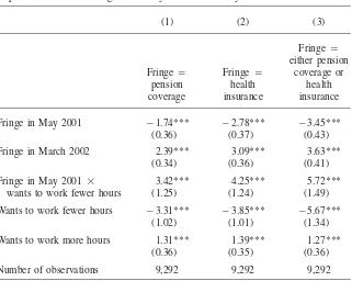
Table 6
Testing the Illusion Hypothesis
Dependent Variable: Change in Weekly Hours from May 2001 to March 2002
(1) (2) (3)
Fringe⳱ pension coverage
Fringe⳱ health insurance
Fringe⳱ either pension
coverage or health insurance
Fringe in May 2001 ⳮ1.74*** ⳮ2.78*** ⳮ3.45***
(0.36) (0.37) (0.43)
Fringe in March 2002 2.39*** 3.09*** 3.63***
(0.34) (0.36) (0.41)
Fringe in May 2001⳯ wants to work fewer hours
3.42*** 4.25*** 5.72***
(1.25) (1.24) (1.49)
Wants to work fewer hours ⳮ3.31*** ⳮ3.85*** ⳮ5.67***
(1.02) (1.01) (1.34)
Wants to work more hours 1.31*** 1.39*** 1.27***
(0.36) (0.35) (0.36)
Number of observations 9,292 9,292 9,292
Note: Matched observations from March 2001, May 2001 and March 2002 Current Population Surveys. Robust standard errors in parentheses. Each regression includes controls for gender, race, age, education, region, initial industry and initial occupation as in Column 4 of Tables 3, 4, and 5. *** 0.01 significance, ** 0.05 significance, * 0.10 significance.
less likely to decrease their hours of work if they have a job with fringe benefits in March 2002. The results are consistent with this prediction.
The crucial variable in testing the illusion of constraints is the interaction between wanting to work less in May 2001 and the presence of fringe benefits. This variable should be positive, indicating that the marginal effect of wanting to work less on subsequent reductions in hours was lower for workers with fringe benefits in May 2001 than for workers without fringe benefits. In effect, this is a difference in dif-ference estimate because both wanting to work less and initial fringe benefits should affect subsequent hours changes, but the model predicts that workers with fringe benefits who want to work less will find it more difficult to reduce hours than we would predict summing the independent effects of initial fringe benefits and wanting to work less.
want-ing to work less is significantly positive in all three regressions. The regression reported in Column 1 defines a fringe benefit as pension coverage and shows that among those without initial pension coverage, the subset who wanted to work fewer hours shed 3.31 more hours than those who were satisfied with their hours. This is consistent with purposeful search. However, looking at the group with initial pension coverage, the outcomes of the subset who said they wanted to work fewer hours (ⳮ1.63⳱ⳮ1.74Ⳮ3.42ⳮ3.31) are essentially the same as the outcomes of the sub-set who were satisfied with their hours (ⳮ1.74).11As the model predicts, workers
may want to work less but jobs with fewer hours they prefer to their current job do not exist because they are economically infeasible. The hours constraints are illusory. This strong prediction of illusion is robust to alternative definitions of fringes (see Columns 2 and 3 of Table 6) and to alternative unreported specifications such as probits on whether hours decreased from May 2001 to March 2002.
To get a sense of what these results might imply about the fraction of constrained workers whose constraints are illusory, consider that workers who have fringe bene-fits and want to work less comprise 21.5 percent of all constrained workers. If the results in Table 6 are read to imply that all of these workers face illusory rather than real constraints, then the frequency of constraints is overstated in the data by about 27 percent. The true fraction will be smaller because even though on average those with fringes who want to work less fail to reduce their hours, some in fact do.
D. Alternative Explanations and Robustness
One alternative interpretation of the results in Tables 3, 4, and 5 is that actual hours are measured with error and fringes are positively correlated with the true value of actual hours. When both actual hours and fringes are included in the regressions, fringes have a positive effect on wanting to work less because they are picking up the part of true actual hours not included in the noisy measure of actual hours. However, in this case, the change in hours estimates in Table 6 would be expected to show that comparing two workers who want to reduce their hours, the one with fringes would reduce his hours more (not less as the model predicts and the estimates in Table 6 show) because that worker would be working more actual hours.
Another seemingly plausible interpretation of these results asserts, correctly, that the observables do not completely control for variations in worker productivity. Since fringes are a normal good, workers with higher truevwill choose more fringes, so that observed fringes will be positively correlated with the unobserved part ofv. If labor supply is backward-bending, high v workers will want to work less and so fringes will be correlated with wanting work less. However, this chain of reasoning is not a satisfying explanation of the empirical results. First, it depends on labor supply being backward-bending, which few cross-sectional studies have found. Sec-ond, it requires labor market frictions, since in a frictionless market workers will find their ideal feasible job, whatever combination of fringes and hours it entails. Even with labor market frictions, the model must explain why higher v workers
(those with fringes in this scenario) have more difficulty getting close to their desired job than lowerv workers (without fringes); that is, why would search frictions be greater for workers with fringe benefits than without?
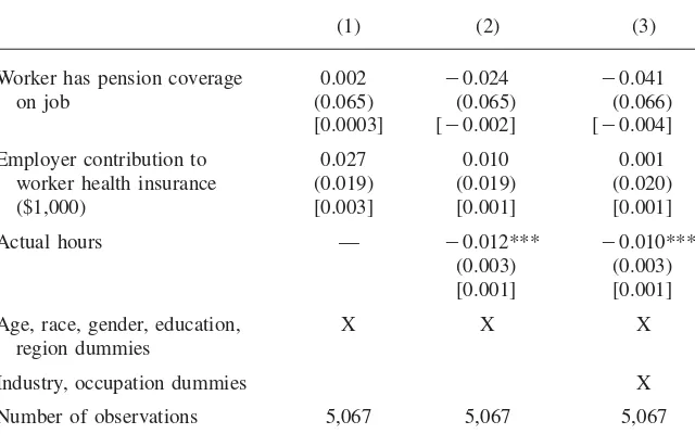
Finally, it could be argued that workers who are paid by the hour respond differently to typical questions about hours constraints than other workers do, because they are used to earnings depending on hours worked. The results reported in Tables 3 – 6 use both hourly-paid workers and those not paid by the hour, although whether a worker is paid hourly is included as a variable in many of the results. To make sure that the results are not sensitive to the inclusion of workers who are not paid by the hour, I report in Appendix Tables A1–A4 estimates parallel to those in Tables 3–6 using only hourly paid workers. Since sample sizes are much smaller (information on whether a worker is paid hourly is missing for many workers), the estimates are less precise but mirror the results using the larger sample of workers in Tables 4–6. Appendix Table A1, which parallels Table 3, fails to find a significant effect of health insurance on wanting to work less, though the estimated effects are all positive.
V. Conclusion
Hours constraints are often interpreted as an indicator of the func-tioning of the labor market because market frictions or imperfections prevent work-ers from attaining feasible jobs with preferred hours of work. Hours constraints are typically identified by worker responses to questions implying that workers consider alternative jobs with more or fewer hours but the same hourly rate of pay, a condition which is intended to restrict the worker to consider only economically feasible jobs. However, jobs with different hours but the same rate of pay may not be feasible when there are complications such as fixed costs of employment, mandatory over-time premia, or fatigue effects. The constraint in those cases may be illusory.
References
Aaronson, Daniel, and Eric French. 2004. “The Effect of Part-Time Work on Wages: Evidence from the Social Security Rules.”Journal of Labor Economics22(2):329–52. Altonji, Joseph, and Christina Paxson. 1988. “Labor Supply Preferences, Hours Constraints
and Hours-Wage Trade-Offs.”Journal of Labor Economics6(2):254–76.
———. 1992. “Labor Supply, Hours Constraints, and Job Mobility.”Journal of Human Resources27(2):256–78.
Beaudry, Paul, and John diNardo. 1995. “Is the Behavior of Hours Worked Consistent with Implicit Contract Theory?”Quarterly Journal of Economics110(3):743–68.
Biddle, Jeff, and Gary Zarkin. 1989. “Choice among Wage-Hours Packages: An Empirical Investigation of Male Labor Supply.”Journal of Labor Economics7(4):415–37. Bloemen, Hans. 2008. “Job Search, Hours Restrictions and Desired Hours of Work.”
Journal of Labor Economics26(1): 137–179.
Blundell, Richard, Mike Brewer, and Marco Francesconi. 2008. “Job Changes and Hours Changes: Understanding the Path of Labor Market Adjustment.”Journal of Labor Economics26(3):421–53.
Cutler, David, and Brigitte Madrian. 1998. “Labor Market Responses to Rising Health Insurance Costs: Evidence on Hours Worked.”Rand Journal of Economics29(3):509–30. Dickens, William, and Shelly Lundberg. 1993. “Hours Restrictions and Labor Supply.”
International Economic Review34(1):169–92.
Ehrenberg, Ronald. 1971.Fringe Benefits and Overtime Behavior.Lexington, Mass.: Heath Lexington Books.
Ham, John. 1982. “Estimation of a Labour Supply Model with Censoring Due to Unemployment and Underemployment.”Review of Economic Studies49(3):339–54. Ham, John and Kevin Reilly. 2002. “Testing Intertemporal Substitution, Implicit Contracts,
and Hours Restriction Models of the Labor Market Using Micro Data.”American Economic Review92(4):905–27.
Hamermesh, Daniel. 1993.Labor Demand. Princeton: Princeton University Press. Kahn, Shulamit and Kevin Lang. 1991. “The Effect of Hours Constraints on Labor Supply
Estimates.”Review of Economics and Statistics73(4): 605–611.
———. 1992. “Constraints on the Choice of Work Hours.”Journal of Human Resources 27(4):661–78.
———. 1995. “The Causes of Hours Constraints: Evidence from Canada.”Canadian Journal of Economics28(4a):914–28.
——— . 1996. “Hours Constraints and the Wage/Hours Locus.”Canadian Journal of Economics29 (Special Issue Part 1): pp. S71-S75.
Lang, Kevin and Shulamit Kahn. 2001. “Hours Constraints: Theory, Evidence and Policy Implications.” InWorking Time in Comparative Perspective, Volume 1,ed. Ging Wong and W. Picot, 261–88. Kalamazoo, Mich.: Upjohn Institute for Employment Research. Rogerson, Richard, and Johanna Wallenius. 2009. “Micro and Macro Elasticities in a Life
Cycle Model with Taxes.”Journal of Economic Theory144(6):2277–92.
Stewart, Mark, and Joanna Swaffield. 1997. “Constraints on the Desired Hours of Work of British Men.”Economic Journal107(441): 520–35.
Appendix
Table A1
Probit Estimates of Hours Constraints: Worker Wants to Work Less (hourly paid workers only)
(1) (2) (3)
Worker has pension coverage on job
0.002 ⳮ0.024 ⳮ0.041
(0.065) (0.065) (0.066)
[0.0003] [ⳮ0.002] [ⳮ0.004]
Employer contribution to worker health insurance ($1,000)
0.027 0.010 0.001
(0.019) (0.019) (0.020)
[0.003] [0.001] [0.001]
Actual hours — ⳮ0.012*** ⳮ0.010***
(0.003) (0.003) [0.001] [0.001]
Age, race, gender, education, region dummies
X X X
Industry, occupation dummies X
Number of observations 5,067 5,067 5,067
Table A2
Probit Estimates of Hours Constraints: Worker Wants to Work More (hourly paid workers only)
(1) (2) (3)
Worker has pension coverage on job
ⳮ0.178*** ⳮ0.171*** ⳮ0.157***
(0.044) (0.044) (0.045)
[ⳮ0.061] [ⳮ0.058] [ⳮ0.054]
Employer contribution to worker health insurance ($1,000)
ⳮ0.035*** ⳮ0.031** ⳮ0.025*
(0.012) (0.013) (0.014)
[ⳮ0.012] [ⳮ0.011] [ⳮ0.001]
Actual hours — ⳮ0.002 ⳮ0.001
(0.001) (0.001) [ⳮ0.001] [ⳮ0.001]
Age, race, gender, education, region dummies
X X X
Industry, occupation dummies
X
Number of observations 5,067 5,067 5,067
Note: Same as Table 3.
Table A3
Ordered Probit Estimates of Hours Constraints (hourly paid workers only)
(1) (2) (3)
Worker has pension coverage on job
ⳮ0.131*** ⳮ0.115*** ⳮ0.102**
(0.038) (0.039) (0.040)
Employer contribution to worker health insurance ($1,000)
ⳮ0.035*** ⳮ0.026** ⳮ0.022*
(0.011) (0.011) (0.012)
Actual hours — ⳮ0.005*** ⳮ0.004***
(0.001) (0.002)
Age, race, gender, education, region dummies
X X X
Industry, occupation dummies X
Number of observations 5,067 5,067 5,067
Table A4
Testing the Illusion Hypothesis (hourly paid workers only)
Dependent Variable: Change in Weekly Hours from May 2001 to March 2002
(1) (2) (3)
Fringe⳱ pension coverage
Fringe⳱ health insurance
Fringe⳱ either pension
coverage or health insurance
Fringe in May 2001 ⳮ0.76 ⳮ2.83*** ⳮ3.18***
(0.62) (0.65) (0.74)
Fringe in March 2002 1.82*** 3.69*** 3.98***
(0.61) (0.65) (0.73)
Fringe in May 2001⳯ wants to work fewer hours
4.00* 6.30*** 7.89***
(2.19) (2.02) (2.25)
Wants to work fewer hours ⳮ2.73 ⳮ4.64*** ⳮ6.78***
(1.69) (1.48) (1.88)
Wants to work more hours 0.59 0.64 0.56
(0.59) (0.58) (0.58)
Number of observations 2,680 2,680 2,680