Interaksi antara tumbuhan dan hewan
di hutan hujan tropis
Andrew J. Marshall
Kuliah LapanaganTaman Nasional Gunung Palung 23 May-3 Juni 2016
• Tipe interaksi antara hewan dan tumbuhan
• Fenologi di hutan tropis
•
Bagaimana habitat mempengaruhi hewan
Interaksi antara tumbuhan
dan hewan
> Tipe interaksi antara hewan dan tumbuhan
• Fenologi di hutan tropis
•
Bagaimana habitat mempengaruhi hewan
Interaksi antara tumbuhan
dan hewan
Tumbuh-tumbuhan “mau” hindari jadi
makanan untuk hewan.
Masukkan beberapa tipe racun dalam daunya,
jadi pemakan daun perlu adaptasi tertentu untuk
melawan rancun-racunan.
Daun: sumber energi untuk tumbuhan
sumber makanan untuk hewan
CO
2O
2
Interaksi antara tumbuhan
dan hewan
Biji: anak pohon
makanan hewan
Interaksi antara tumbuhan
dan hewan
Tumbuh-tumbuhan “mau” hindari anaknya jadi
makanan untuk hewan.
Masukkan beberapa tipe racun dalam biji atau
bikin biji keras sekali, jadi pemakan daun perlu
adaptasi tertentu untuk melawan rancun-racunan.
Buah: strategi untuk penyebar biji
sumber makanan untuk hewan
Interaksi antara tumbuhan
dan hewan
Kerja sama!
Tumbuh-tumbuhan “mau” buah dimakan
hewan (asal biji tetap utuh).
sumber: Phillips & Phillips 2016
Dibawa…
Burung kecil
buah kecil, tidak berbau
berkilauan, merah atau hitam
daging manis, kulit lembek
biji kecil, licin
sumber: Phillips & Phillips 2016
Dibawa…
Burung kecil
Burung enggang
tidak berbau
kulut tebal dan keras
pecah belah
sumber: Phillips & Phillips 2016
Dibawa…
Burung kecil
Burung enggang
Primata
wangi
masak warna tua/tidak berkilau
kulit tebal
daging manis, tempel ke biji
biji agak besar (~2 cm)
sumber: Phillips & Phillips 2016
Dibawa…
Burung kecil
Burung enggang
Primata
Tikus
biji besar, keras, berkilau
biji agak beracun
kulit tebal
tanpa daging
sumber: Phillips & Phillips 2016
Dibawa…
Burung kecil
Burung enggang
Primata
Tikus
Gajah
sangat wangi dan besar
berbuah di pohon kecil
kulit tebal
sumber: Phillips & Phillips 2016
sumber: Phillips & Phillips 2016
sumber: Phillips & Phillips 2016
sumber: Phillips & Phillips 2016
sumber: Phillips & Phillips 2016
Dibawa mamalia besar
Kalau punah, gimana?
Dibawa air
Vatica resak
Barringtonia sarchostachys
Dipetrocarpaceae
Uncaria
sp.
• Tipe interaksi antara hewan dan tumbuhan
> Fenologi di hutan tropis
•
Bagaimana habitat mempengaruhi hewan
Interaksi antara tumbuhan
dan hewan
Fenologi hutan tropis
0
2
4
6
8
10
12
14
16
Ja
n
8
6
Ap
r
8
6
Ju
l
8
6
O
ct
8
6
Ja
n
8
7
Ap
r
8
7
Ju
l
8
7
O
ct
8
7
Ja
n
8
8
Ap
r
8
8
Ju
l
8
8
O
ct
8
8
Ja
n
8
9
Ap
r
8
9
Ju
l
8
9
O
ct
8
9
Ja
n
9
0
Ap
r
9
0
Ju
l
9
0
O
ct
9
0
Ja
n
9
1
Ap
r
9
1
Ju
l
9
1
T
F
A
(p
a
tch
e
s/
h
a
)
0
2
4
6
8
10
12
14
16
#
t
a
xa
w
it
h
f
ru
it
A
Marshall (2004)0 % 10% 20% 30% 40% 50% 60% 70% 80% 90% 100% Jan-Mar 86 (31) Apr-Ju n 86 (36) Jul-Se p 86 (19) Oc t-Dec 86 (35) Jan-Mar 87 (28) Apr-Ju n 87 (14) Jul-Se p 87 (25) Oc t-Dec 87 (57) Jan-Mar 88 (45) Apr-Ju n 88 (49) Jul-Se p 88 (12) Oc t-Dec 88 (21) Jan-Mar 89 (12) Apr-Ju n 89 (4) Jul-Se p 89 (26) Oc t-Dec 89 (29) Jan-Mar 90 (28) Apr-Ju n 90(27) Jul-Se p 90 (17) Oc t-Dec 90 (13) Jan-Mar 91 (8) % total fe eding observ ation s Leaves Figs
Fruit pulp+ seeds Flowers
% Feeding Observations
% Feeding Observations
time
time
kelempiau
0 % 10% 20% 30% 40% 50% 60% 70% 80% 90% 100% Jan-Mar 86 (38) Apr-Jun 86 (57) Jul-Se p 86 (26) Oc t-Dec 86 (35) Jan-Mar 87 (49) Apr-Ju n 87 (320) Jul-Se p 87 (71) Oc t-Dec 87 (45) Jan-Mar 88 (40) Apr-Jun 88 (37) Jul-Se p 88 (24) Oc t-Dec 88 (24) Jan-Mar 89 (18) Apr-Jun 89 (8) Jul-Se p 89 (11) Oc t-Dec 89 (25) Jan-Mar 90 (15) Apr-Jun 90 (15) Jul-Se p 90 (13) Oc t-Dec 90 (13) Jan-Mar 91 (11)%
total
fe
eding
observ
ation
s
Seeds Leaves Figs Fruit pulp Flowerskelasi
time
time
% of
diet
% of
diet
Fenologi hutan tropis
Perbandingan antara lokasi dan
tipe hutan
Fenologi hutan tropis
Perbandingan antara lokasi dan
tipe hutan
Sumatra
Sumatra
Borneo
Borneo
Tujuh tipe hutan
tanah, ketinggian, cuaca -> jenis tumbuhan berbeda
Satsiun Penelitian Cabang Panti
% tree species shared with another habitat types PS FS AB LS LG UG MO
max 11 19 22 22 15 14 10 mean 9.5 15 16.5 16 11.5 10.5 8.5 min 8 11 11 10 8 7 7 5 10 15 20 !"#$ %"#$ &"#$ '"#$ ("#$ #"#$ )"#$ *"#$ % tree species shared with other habitats (max, mean, & min; pairwise comparisons among habitats) UB Ridge GP ridge
Average STDEV Average STDEV
DT 5-max 30.13404255 1.454735728 SK 2-max 30.65558621 2.3872342 DT 5-min 22.84042553 0.738273871 SK 2-min 22.71551724 1.314934689 DT 5-hujan 143.0340426 118.8802679 SK 2-hujan 121.8651724 100.1716091 DR 11-max 30.10638298 1.317340682 SC 7-max 31.23684211 2.232281951 DR 11-min 22.23404255 3.138836518 SC 7-min 22.66896552 0.855161193 DR 11-hujan 130.2404255 102.4921281 SC 7-hujan 121.4806897 105.3540278 UB 15-max 30.26702128 2.364840334 GP 35-max 30.60344828 1.541128035 UB 15-min 21.72340426 1.58693336 GP 35-min 25.6637931 26.39367746 UB 15-hujan 143.3744681 128.8278397 GP 35-hujan 113.3768966 95.06716228 NB13-max 28.00106383 1.373386185 TK 22-max 29.37931034 1.897159337 NB13-min 21.17021277 0.890434948 TK 22-min 21.56896552 1.95216541 NB13-hujan 126.7765957 87.91246055 TK 22-hujan 101.96 85.65333369 UB 53-max 28.60957447 9.626065472 MR 2-max 27.69827586 0.922143076 UB 53-min 20.91489362 0.722398715 MR 2-min 21.73275862 1.490365307 UB 53-hujan 117.9940426 85.10232875 MR 2-hujan 121.477931 93.26856545 UB 73-max 24.9787234 1.929180948 GP 80-max 28.74655172 2.065014805 UB 73-min 19.28723404 1.025814158 GP 80-min 20.95689655 1.060802753 UB 73-hujan 131.5978723 96.87636705 GP 80-hujan 107.7993103 85.38255683 UB 88-max 26.92391304 2.216020937 GP 90-max 26.3362069 1.292311716 UB 88-min 17.35869565 1.319356087 GP 90-min 19.47413793 1.268451238 UB 88-hujan 126.1630435 91.1153856 GP 90-hujan 107.3596552 84.9438494 PS FS AB LS Max temp 30.39481438 30.67161254 30.43523478 28.69018709 Min temp 22.77797139 30.43523478 23.69359868 21.36958914 133.9043432 127.1778983 130.7405227 rainfall 132.4496075 125.8605576 128.3756823 114.3682979 130.9948718 122.7217211 -0.452157413 !!"# !$%# !&"# "'%# !'%# $'%# ('%# &'%# %'%# )'%# *'%# UB Ridge GP ridge
Average STDEV Average STDEV DT 5-max 30.13404255 1.454735728 SK 2-max 30.65558621 2.3872342 DT 5-min 22.84042553 0.738273871 SK 2-min 22.71551724 1.314934689 DT 5-hujan 143.0340426 118.8802679 SK 2-hujan 121.8651724 100.1716091 DR 11-max 30.10638298 1.317340682 SC 7-max 31.23684211 2.232281951 DR 11-min 22.23404255 3.138836518 SC 7-min 22.66896552 0.855161193 DR 11-hujan 130.2404255 102.4921281 SC 7-hujan 121.4806897 105.3540278 UB 15-max 30.26702128 2.364840334 GP 35-max 30.60344828 1.541128035 UB 15-min 21.72340426 1.58693336 GP 35-min 25.6637931 26.39367746 UB 15-hujan 143.3744681 128.8278397 GP 35-hujan 113.3768966 95.06716228 NB13-max 28.00106383 1.373386185 TK 22-max 29.37931034 1.897159337 NB13-min 21.17021277 0.890434948 TK 22-min 21.56896552 1.95216541 NB13-hujan 126.7765957 87.91246055 TK 22-hujan 101.96 85.65333369 UB 53-max 28.60957447 9.626065472 MR 2-max 27.69827586 0.922143076 UB 53-min 20.91489362 0.722398715 MR 2-min 21.73275862 1.490365307 UB 53-hujan 117.9940426 85.10232875 MR 2-hujan 121.477931 93.26856545 UB 73-max 24.9787234 1.929180948 GP 80-max 28.74655172 2.065014805 UB 73-min 19.28723404 1.025814158 GP 80-min 20.95689655 1.060802753 UB 73-hujan 131.5978723 96.87636705 GP 80-hujan 107.7993103 85.38255683 UB 88-max 26.92391304 2.216020937 GP 90-max 26.3362069 1.292311716 UB 88-min 17.35869565 1.319356087 GP 90-min 19.47413793 1.268451238 UB 88-hujan 126.1630435 91.1153856 GP 90-hujan 107.3596552 84.9438494 PS FS AB LS Max temp 30.39481438 30.67161254 30.43523478 28.69018709 Min temp 22.77797139 30.43523478 23.69359868 21.36958914 133.9043432 127.1778983 130.7405227 rainfall 132.4496075 125.8605576 128.3756823 114.3682979 130.9948718 122.7217211 -0.452157413 !!"# !$%# !&"# "'%# !'%# $'%# ('%# &'%# %'%# )'%# *'%# !+# $&# ("# ()# "'%# !'%# $'%# ('%# &'%# %'%# )'%# *'%# max, min temperature (10 day period, C) PS FS AB LS LG UG MO avg rainfall (10 day period, mm) FOREST TYPES
0 2 4 6 8 10 12 14 16
Ja
n
86
Ap
r 8
6
Ju
l 8
6
Oct
8
6
Ja
n
87
Ap
r 8
7
Ju
l 8
7
Oct
8
7
Ja
n
88
Ap
r 8
8
Ju
l 8
8
Oct
8
8
Ja
n
89
Ap
r 8
9
Ju
l 8
9
Oct
8
9
Ja
n
90
Ap
r 9
0
Ju
l 9
0
Oct
9
0
Ja
n
91
Ap
r 9
1
Ju
l 9
1
TF
A
(p
at
ch
es/
ha
)
0 2 4 6 8 10 12 14 16#
ta
xa
w
ith
fru
it
A
Hutan dataran rendah
0 2 4 6 8 10 12 14 16 18 20
Ja
n 8
6
Ap
r 8
6
Ju
l 8
6
Oct
86
Ja
n 8
7
Ap
r 8
7
Ju
l 8
7
Oct
87
Ja
n 8
8
Ap
r 8
8
Ju
l 8
8
Oct
88
Ja
n 8
9
Ap
r 8
9
Ju
l 8
9
Oct
89
Ja
n 9
0
Ap
r 9
0
Ju
l 9
0
Oct
90
Ja
n 9
1
Ap
r 9
1
Ju
l 9
1
TF
A
(pa
tch
es/
ha
)
0 0.5 1 1.5 2 2.5 3 3.5 4 4.5# t
axa
w
ith
fru
it
Pegununungan
0 2 4 6 8 10 12 14Ja
n
86
Ap
r 8
6
Ju
l 8
6
O
ct
8
6
Ja
n
87
Ap
r 8
7
Ju
l 8
7
O
ct
8
7
Ja
n
88
Ap
r 8
8
Ju
l 8
8
O
ct
8
8
Ja
n
89
Ap
r 8
9
Ju
l 8
9
O
ct
8
9
Ja
n
90
Ap
r 9
0
Ju
l 9
0
O
ct
9
0
Ja
n
91
Ap
r 9
1
Ju
l 9
1
TF
A
(p
at
ch
es/
ha
)
0 2 4 6 8 10 12 14#
ta
xa
w
ith
fru
it
Jumlah sumber makan kelempiau
Rawa gambut
Musim buah raya Bulan dgn banyak buah Bulan dgn sedikit buah Musim kelaparan Jumlah tipe makan ygFenologi hutan tropis
Perbandingan antara lokasi dan
tipe hutan
0 2 4 6 8 10 12 14 16 Jan 86 Apr 86 Jul 86 Oc t 86 Jan 87 Apr 87 Jul 87 Oc t 87 Jan 88 Apr 88 Jul 88 Oc t 88 Jan 89 Apr 89 Jul 89 Oc t 89 Jan 90 Apr 90 Jul 90 Oc t 90 Jan 91 Apr 91 Jul 91
Jumlah pohon makanan per ha
Waktu (tahun)
Sumber makanan kelasi, Jan. 1986 - Okt. 91
musim kelaparan
1986
1987
1988
1989
1990
1991
Marshall 2004
Cannon, Curran, Marshall & Leighton 2007
Ecol. Lett.
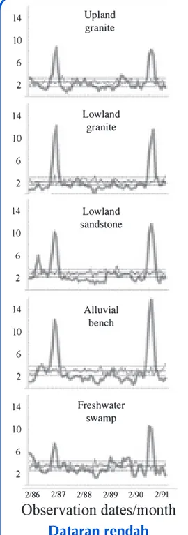
granite climbers (Fig. S3), variability in reproductive pro-ductivity is quite high. In the lowland sandstone, climbers were the most consistently reproductive, ranking substan-tially higher than all other forest types across the observa-tion period. This high relative rank is largely due to the very
low variability in reproductive productivity as the mean and maximum productivity values for the lowland sandstone are quite low. The freshwater swamp climber community was the second most consistently reproductive of the seven forest types examined.
(a) (h) (b) (i) (c) (j) (d) (k) (e) (l) (f) (m) (g) (n)
Figure 4 Fruiting behaviour over
68 months in a Bornean rainforest for different forest types. (a) montane (mean N month)1 = 283, min = 266, max = 301); (b) upper granite (mean Nmonth)1 = 640, min = 504, max = 678); (c) lower granite (mean N month)1= 673, min = 572, max = 696); (d) lower sandstone (mean N month)1 = 1023, min = 911, max = 1049); (e) alluvial bench (mean Nmonth)1 = 646, min = 578, max = 671); (f) freshwa-ter swamp (mean Nmonth)1 = 870, min = 676, max = 922); and (g) peat swamp (mean N month)1= 688, min = 610, max = 701). Observed values are shown in thick grey line. The average level of fruiting expected across all months is indicated by the solid black line while 95% confidence limits are shown by the dashed black lines. The thin grey line illustrates a single replicate of random fruiting behaviour. Frequency distribution of reproductive levels by month follow: (h) montane; (i) upper granite; (j) lower granite; (k) lower sandstone; (l) alluvial bench; (m) freshwater swamp; and (n) peat swamp. Barcharts illustrate observed levels of reproduction. Black curves assume a single season, grey curves assume a mixed model with two seasons.
Letter Landscape level Bornean plant reproduction 963
!2007 Blackwell Publishing Ltd/CNRS
granite climbers (Fig. S3), variability in reproductive
pro-ductivity is quite high. In the lowland sandstone, climbers
were the most consistently reproductive, ranking
substan-tially higher than all other forest types across the
observa-tion period. This high relative rank is largely due to the very
low variability in reproductive productivity as the mean and
maximum productivity values for the lowland sandstone are
quite low. The freshwater swamp climber community was
the second most consistently reproductive of the seven
forest types examined.
(a) (h) (b) (i) (c) (j) (d) (k) (e) (l) (f) (m) (g) (n)
Figure 4 Fruiting behaviour over
68 months in a Bornean rainforest for different forest types. (a) montane (mean
Nmonth)1 = 283, min = 266, max = 301);
(b) upper granite (meanN month)1 = 640,
min = 504, max = 678); (c) lower granite
(mean N month)1 = 673, min = 572, max
= 696); (d) lower sandstone (mean
Nmonth)1 = 1023, min = 911, max =
1049); (e) alluvial bench (mean N month)1
= 646, min = 578, max = 671); (f)
freshwa-ter swamp (mean N month)1 = 870,
min = 676, max = 922); and (g) peat swamp
(mean N month)1 = 688, min = 610,
max = 701). Observed values are shown in thick grey line. The average level of fruiting expected across all months is indicated by the solid black line while 95% confidence limits are shown by the dashed black lines. The thin grey line illustrates a single replicate of random fruiting behaviour. Frequency distribution of reproductive levels by month follow: (h) montane; (i) upper granite; (j) lower granite; (k) lower sandstone; (l) alluvial bench; (m) freshwater swamp; and (n) peat swamp. Barcharts illustrate observed levels of reproduction. Black curves assume a single season, grey curves assume a mixed model with two seasons.
Letter Landscape level Bornean plant reproduction 963
! 2007 Blackwell Publishing Ltd/CNRS
Dataran rendah
Gambut
granite climbers (Fig. S3), variability in reproductive pro-ductivity is quite high. In the lowland sandstone, climbers were the most consistently reproductive, ranking substan-tially higher than all other forest types across the observa-tion period. This high relative rank is largely due to the very
low variability in reproductive productivity as the mean and maximum productivity values for the lowland sandstone are quite low. The freshwater swamp climber community was the second most consistently reproductive of the seven forest types examined.
(a) (h) (b) (i) (c) (j) (d) (k) (e) (l) (f) (m) (g) (n)
Figure 4 Fruiting behaviour over 68 months in a Bornean rainforest for different forest types. (a) montane (mean
N month)1 = 283, min = 266, max = 301); (b) upper granite (mean N month)1 = 640, min = 504, max = 678); (c) lower granite (mean Nmonth)1 = 673, min = 572, max = 696); (d) lower sandstone (mean
N month)1 = 1023, min = 911, max = 1049); (e) alluvial bench (mean Nmonth)1 = 646, min = 578, max = 671); (f) freshwa-ter swamp (mean N month)1 = 870, min = 676, max = 922); and (g) peat swamp (mean N month)1= 688, min = 610, max = 701). Observed values are shown in thick grey line. The average level of fruiting expected across all months is indicated by the solid black line while 95% confidence limits are shown by the dashed black lines. The thin grey line illustrates a single replicate of random fruiting behaviour. Frequency distribution of reproductive levels by month follow: (h) montane; (i) upper granite; (j) lower granite; (k) lower sandstone; (l) alluvial bench; (m) freshwater swamp; and (n) peat swamp. Barcharts illustrate observed levels of reproduction. Black curves assume a single season, grey curves assume a mixed model with two seasons.
Letter Landscape level Bornean plant reproduction 963
!2007 Blackwell Publishing Ltd/CNRS
granite climbers (Fig. S3), variability in reproductive pro-ductivity is quite high. In the lowland sandstone, climbers were the most consistently reproductive, ranking substan-tially higher than all other forest types across the observa-tion period. This high relative rank is largely due to the very
low variability in reproductive productivity as the mean and maximum productivity values for the lowland sandstone are quite low. The freshwater swamp climber community was the second most consistently reproductive of the seven forest types examined.
(a) (h) (b) (i) (c) (j) (d) (k) (e) (l) (f) (m) (g) (n)
Figure 4 Fruiting behaviour over 68 months in a Bornean rainforest for different forest types. (a) montane (mean
Nmonth)1 = 283, min = 266, max = 301); (b) upper granite (mean N month)1= 640, min = 504, max = 678); (c) lower granite (mean N month)1= 673, min = 572, max = 696); (d) lower sandstone (mean
Nmonth)1 = 1023, min = 911, max = 1049); (e) alluvial bench (mean N month)1 = 646, min = 578, max = 671); (f) freshwa-ter swamp (mean N month)1= 870, min = 676, max = 922); and (g) peat swamp (mean N month)1= 688, min = 610, max = 701). Observed values are shown in thick grey line. The average level of fruiting expected across all months is indicated by the solid black line while 95% confidence limits are shown by the dashed black lines. The thin grey line illustrates a single replicate of random fruiting behaviour. Frequency distribution of reproductive levels by month follow: (h) montane; (i) upper granite; (j) lower granite; (k) lower sandstone; (l) alluvial bench; (m) freshwater swamp; and (n) peat swamp. Barcharts illustrate observed levels of reproduction. Black curves assume a single season, grey curves assume a mixed model with two seasons.
Letter Landscape level Bornean plant reproduction 963
!2007 Blackwell Publishing Ltd/CNRS
granite climbers (Fig. S3), variability in reproductive
pro-ductivity is quite high. In the lowland sandstone, climbers
were the most consistently reproductive, ranking
substan-tially higher than all other forest types across the
observa-tion period. This high relative rank is largely due to the very
low variability in reproductive productivity as the mean and
maximum productivity values for the lowland sandstone are
quite low. The freshwater swamp climber community was
the second most consistently reproductive of the seven
forest types examined.
(a) (h) (b) (i) (c) (j) (d) (k) (e) (l) (f) (m) (g) (n)
Figure 4 Fruiting behaviour over
68 months in a Bornean rainforest for different forest types. (a) montane (mean
N month)1 = 283, min = 266, max = 301);
(b) upper granite (mean N month)1 = 640,
min = 504, max = 678); (c) lower granite
(mean N month)1 = 673, min = 572, max
= 696); (d) lower sandstone (mean
N month)1 = 1023, min = 911, max =
1049); (e) alluvial bench (mean N month)1
= 646, min = 578, max = 671); (f)
freshwa-ter swamp (mean N month)1 = 870,
min = 676, max = 922); and (g) peat swamp
(mean N month)1 = 688, min = 610,
max = 701). Observed values are shown in thick grey line. The average level of fruiting expected across all months is indicated by the solid black line while 95% confidence limits are shown by the dashed black lines. The thin grey line illustrates a single replicate of random fruiting behaviour. Frequency distribution of reproductive levels by month follow: (h) montane; (i) upper granite; (j) lower granite; (k) lower sandstone; (l) alluvial bench; (m) freshwater swamp; and (n) peat swamp. Barcharts illustrate observed levels of reproduction. Black curves assume a single season, grey curves assume a mixed model with two seasons.
Letter Landscape level Bornean plant reproduction 963
!2007 Blackwell Publishing Ltd/CNRS
Pegunungan
Liana
Ficus
Pohon
kecil
Pohon
besar
Cannon, Curran, Marshall & Leighton 2007
Ecol. Lett.
berbuah
raya
(rata-rata)
tidak
0 5 1 0 1 5 2 0 2 5 3 0 Feb 8 6 May 86 Aug 8 6 Nov 8 6 Feb 8 7 May 87 Aug 8 7 Nov 8 7 Feb 8 8 May 88 Aug 8 8 Nov 8 8 Feb 8 9 May 89 Aug 8 9 Nov 8 9 Feb 9 0 May 90 Aug 9 0 Nov 9 0 Feb 9 1 May 91 Aug 9 1 0 5 1 0 1 5 2 0 2 5 3 0 Feb 8 6 May 86 Aug 8 6 Nov 8 6 Feb 8 7 May 87 Aug 8 7 Nov 8 7 Feb 8 8 May 88 Aug 8 8 Nov 8 8 Feb 8 9 May 89 Aug 8 9 Nov 8 9 Feb 9 0 May 90 Aug 9 0 Nov 9 0 Feb 9 1 May 91 Aug 9 1
Musim buah raya
Musim berbuah biasa
Neoscortechinia kingii
Rourea major
0 5 1 0 1 5 2 0 2 5 3 0 Feb 8 6 May 86 Aug 8 6 Nov 8 6 Feb 8 7 May 87 Aug 8 7 Nov 8 7 Feb 8 8 May 88 Aug 8 8 Nov 8 8 Feb 8 9 May 89 Aug 8 9 Nov 8 9 Feb 9 0 May 90 Aug 9 0 Nov 9 0 Feb 9 1 May 91 Aug 9 1Porterandia sessiliflora
Musim buah sedikit
time
time
time
Food/ha
Food/ha
Food/ha
Berbuah raya v. musim-musim tertentu
Average rainfall, Davis, CA 1930–2010 weather.com
Konjup, Southwest Australia Hill & Donald 2003
New South Wales, Australia
Average rainfall, Ann Arbor, MI 1930–2010
weather.com
Average rainfall, Davis, CA 1930–2010
weather.com
Berbuah raya v. musim-musim tertentu
musim-musim tertentu
Landscape level Bornean plant reproduction, Cannon et al. figures
Figure S1. Annual reproductive behavior of all woody plants. Monthly observations are plotted for each year of the percentage of the reproductive stems. Each year is indicated by a different type of line, as shown in the legend.
persen tumbuhan yg berbuah
Cannon, Curran, Marshall & Leighton (2007) Ecology Letters
Feb
Apr
Jun
Aug
Oct
Dec
Monthly observations (excluding masts)
2%
3%
4%
1990 1990 1986 1987 1991 1991 1986 1988 1988 1989 1989 1987Berbuah raya v. musim-musim tertentu
El Niño Southern Oscillation (ENSO) years
Seed exports
(millions of kg of dry mass)
ENSO
Non- ENSO
Year
June–Sept r
ainfall (mm)
• Tipe interaksi antara hewan dan tumbuhan
• Fenologi di hutan tropis
>
Bagaimana habitat mempengaruhi hewan
Interaksi antara tumbuhan
dan hewan
Kelempiau
(Hylobates albibarbis)
•
Berat badan 5-6 kg
•
Menjaga wilayah sebesar
30-40 ha
•
2-7 individu per kelompok
•
satu laki-laki kawin sama satu betina
•
Berat badan 5.5-7 kg
•
Wilayah sebesar 70-85 ha
T. Laman
T. Laman
•
2-11 individu per kelompok
•
satu laki-laki bisa kawin sama lebih dari satu betina
Kelasi
Dua jenis ini merupahkan contoh bagus
untuk meneliti pertanyaan ekologi karena:
• banyak informasi tentang jenis
2
binatang ini sudah
tersedia dari SPCP dan tempat lain
• hewan
2
tersebut mentempati beberapa macam hutan
• berat badan hampir sama, tapi makanan dan sistem sosial
jauh beda
• hewan
2
ini menjaga wilayah, dan tidak merantau ke
tempat lain untuk cari makanan (seperti orangutan), jadi
efek-efek kwalitas habitat lebih jelas dan mudah dilihat
• kepadatan cukup tinggi, berarti dapat ambil sampel yang
Marshall, Beaudrot & Wittmer (2014) Inter. J. Primatol.
covariates contribute to any top models (all models including phenology had
Δ
AIC > 3
and model weight < 0.15).
0 15 30 Macaca CVSPACE = 1.55 0 1 2 Callosciurus CVSPACE = 0.80 0 1.5 3 Ratufa CVSPACE = 0.66 0 2 4 Sus CVSPACE = 0.65 0 2 4 Pongo CVSPACE = 0.59 0 7.5 15 Hylobates CVSPACE = 0.58 0 7.5 15 Presbytis CVSPACE = 0.57 0 1.5 3 B. rhinoceros CVSPACE = 0.55 0 1.5 3 Anorrhinus CVSPACE = 0.51
AB.II AB.I LS.II FS.I LS.I PS.I LG.II LG.I UG.II UG.I MO.I MO.II 0 0.25 0.5 B. vigil CVSPACE= 0.37 Habitat partitions Population density +/ − SE (individuals/km 2 )
Fig. 3
Spatial variation in frugivore population densities at the Cabang Panti Research Station, Gunung
Palung National Park, West Kalimantan from October 2007 to February 2013. Mean (±SE) model averaged
population density (individuals/km
2) for each vertebrate frugivore by habitat partition (
D
SPACE). Note that the
y
-axis scale differs among plots, therefore the height of bars reflects relative habitat quality of partitions within
each taxon. The highest partition specific mean population density for each taxon is shown with a black bar,
second highest in dark gray, third highest in light gray, and all others in white. Taxon names are given on the
right side of the figure, along with the coefficient of variation for model averaged population density among
partitions (CV
SPACE, an index of habitat specialization). Species are listed from top to bottom in descending
order of habitat specialization; habitat partitions are listed from left to right in descending order of mean
population density for the 10 frugivore species shown. Lowland forest types contain the highest densities of all
10 frugivorous species.
Responses of Primates to Plant Resource Variability
covariatescontributetoanytopmodels(allmodelsincludingphenologyhad
Δ
AIC>3
and model weight < 0.15).
0
15
30
Macaca
CV
SPACE= 1.55
0
1
2
Callosciurus
CV
SPACE= 0.80
0
1.5
3
Ratufa
CV
SPACE= 0.66
0
2
4
Sus
CV
SPACE= 0.65
0
2
4
Pongo
CV
SPACE= 0.59
0
7.5
15
Hylobates
CV
SPACE= 0.58
0
7.5
15
Presbytis
CV
SPACE= 0.57
0
1.5
3
B. rhinoceros
CV
SPACE= 0.55
0
1.5
3
Anorrhinus
CV
SPACE= 0.51
AB.II
AB.I
LS.II
FS.I
LS.I
PS.I
LG.II
LG.I
UG.II
UG.I
MO.I
MO.II
0
0.25
0.5
B. vigil
CV
SPACE= 0.37
Habitat partitions
Population density +/ − SE (individuals/km 2 )Fig. 3
Spatial variation in frugivore population densities at the Cabang Panti Research Station, Gunung
Palung National Park, West Kalimantan from October 2007 to February 2013. Mean (±SE) model averaged
populationdensity(individuals/km
2
)foreachvertebratefrugivorebyhabitatpartition(
D
SPACE
).Notethatthe
y
-axisscalediffersamongplots,thereforetheheightofbarsreflectsrelativehabitatqualityofpartitionswithin
each taxon. The highest partition specific mean population density for each taxon is shown with a black bar,
second highest in darkgray, third highestin light gray, and all othersin white. Taxon namesaregivenon the
right side of the figure, along with the coefficient of variation for model averaged population density among
partitions (CV
SPACE
, an index of habitat specialization). Species are listed from top to bottom in descending
order of habitat specialization; habitat partitions are listed from left to right in descending order of mean
populationdensityforthe10frugivorespeciesshown.Lowlandforesttypescontainthehighestdensitiesofall
10 frugivorous species.
Responses of Primates to Plant Resource Variability
covariatescontributetoanytopmodels(allmodelsincludingphenologyhad
ΔAIC>3
and model weight < 0.15).
0
15
30
Macaca
CV
SPACE= 1.55
0
1
2
Callosciurus
CV
SPACE= 0.80
0
1.5
3
Ratufa
CV
SPACE= 0.66
0
2
4
Sus
CV
SPACE= 0.65
0
2
4
Pongo
CV
SPACE= 0.59
0
7.5
15
Hylobates
CV
SPACE= 0.58
0
7.5
15
Presbytis
CV
SPACE= 0.57
0
1.5
3
B. rhinoceros
CV
SPACE= 0.55
0
1.5
3
Anorrhinus
CV
SPACE= 0.51
AB.II
AB.I
LS.II
FS.I
LS.I
PS.I
LG.II
LG.I
UG.II
UG.I
MO.I
MO.II
0
0.25
0.5
B. vigil
CV
SPACE= 0.37
Habitat partitions
Population density +/ − SE (individuals/km 2 )Fig. 3
Spatial variation in frugivore population densities at the Cabang Panti Research Station, Gunung
Palung National Park, West Kalimantan from October 2007 to February 2013. Mean (±SE) model averaged
population density (individuals/km
2
) for eachvertebratefrugivoreby habitat partition(
D
SPACE
).Note that the
y
-axisscalediffersamongplots,thereforetheheightofbarsreflectsrelativehabitatqualityofpartitionswithin
each taxon. The highest partition specific mean population density for each taxon is shown with a black bar,
second highest in dark gray, third highest in light gray, and all others in white. Taxon names are given on the
right side of the figure, along with the coefficient of variation for model averaged population density among
partitions (CV
SPACE
, an index of habitat specialization). Species are listed from top to bottom in descending
order of habitat specialization; habitat partitions are listed from left to right in descending order of mean
populationdensityforthe10frugivorespeciesshown.Lowlandforesttypescontainthehighestdensitiesofall
10 frugivorous species.
Responses of Primates to Plant Resource Variability
Kepadatan
(individu/km
2)
Kelempiau
Kelasi
Bagian tipe hutan
Kwalitas habitat berbeda
covariates contribute to any top models (all models including phenology hadΔAIC > 3
and model weight < 0.15).
0 15 30 Macaca CVSPACE = 1.55 0 1 2 Callosciurus CVSPACE = 0.80 0 1.5 3 Ratufa CVSPACE = 0.66 0 2 4 Sus CVSPACE = 0.65 0 2 4 Pongo CVSPACE = 0.59 0 7.5 15 Hylobates CVSPACE = 0.58 0 7.5 15 Presbytis CVSPACE = 0.57 0 1.5 3 B. rhinoceros CVSPACE = 0.55 0 1.5 3 Anorrhinus CVSPACE = 0.51
AB.II AB.I LS.II FS.I LS.I PS.I LG.II LG.I UG.II UG.I MO.I MO.II 0 0.25 0.5 B. vigil CVSPACE= 0.37 Habitat partitions Population density +/ − SE (individuals/km 2 )
Fig. 3 Spatial variation in frugivore population densities at the Cabang Panti Research Station, Gunung Palung National Park, West Kalimantan from October 2007 to February 2013. Mean (±SE) model averaged population density (individuals/km2) for each vertebrate frugivore by habitat partition (D
SPACE). Note that the
y-axis scale differs among plots, therefore the height of bars reflects relative habitat quality of partitions within each taxon. The highest partition specific mean population density for each taxon is shown with a black bar, second highest in dark gray, third highest in light gray, and all others in white. Taxon names are given on the right side of the figure, along with the coefficient of variation for model averaged population density among partitions (CVSPACE, an index of habitat specialization). Species are listed from top to bottom in descending
order of habitat specialization; habitat partitions are listed from left to right in descending order of mean population density for the 10 frugivore species shown. Lowland forest types contain the highest densities of all 10 frugivorous species.
1188 A.J. Marshall et al.
covariates contribute to any top models (all models including phenology hadΔAIC > 3 and model weight < 0.15).
0 15 30 Macaca CVSPACE = 1.55 0 1 2 Callosciurus CVSPACE = 0.80 0 1.5 3 Ratufa CVSPACE = 0.66 0 2 4 Sus CVSPACE = 0.65 0 2 4 Pongo CVSPACE = 0.59 0 7.5 15 Hylobates CVSPACE = 0.58 0 7.5 15 Presbytis CVSPACE = 0.57 0 1.5 3 B. rhinoceros CVSPACE = 0.55 0 1.5 3 Anorrhinus CVSPACE = 0.51
AB.II AB.I LS.II FS.I LS.I PS.I LG.II LG.I UG.II UG.I MO.I MO.II 0 0.25 0.5 B. vigil CVSPACE= 0.37 Habitat partitions Population density +/ − SE (individuals/km 2 )
Fig. 3 Spatial variation in frugivore population densities at the Cabang Panti Research Station, Gunung Palung National Park, West Kalimantan from October 2007 to February 2013. Mean (±SE) model averaged population density (individuals/km2) for each vertebrate frugivore by habitat partition (DSPACE). Note that the y-axis scale differs among plots, therefore the height of bars reflects relative habitat quality of partitions within each taxon. The highest partition specific mean population density for each taxon is shown with a black bar, second highest in dark gray, third highest in light gray, and all others in white. Taxon names are given on the right side of the figure, along with the coefficient of variation for model averaged population density among partitions (CVSPACE, an index of habitat specialization). Species are listed from top to bottom in descending
order of habitat specialization; habitat partitions are listed from left to right in descending order of mean population density for the 10 frugivore species shown. Lowland forest types contain the highest densities of all 10 frugivorous species.
1188 A.J. Marshall et al.
covariates contribute to any top models (all models including phenology hadΔAIC > 3 and model weight < 0.15).
0 15 30 Macaca CVSPACE = 1.55 0 1 2 Callosciurus CVSPACE = 0.80 0 1.5 3 Ratufa CVSPACE = 0.66 0 2 4 Sus CVSPACE = 0.65 0 2 4 Pongo CVSPACE = 0.59 0 7.5 15 Hylobates CVSPACE = 0.58 0 7.5 15 Presbytis CVSPACE = 0.57 0 1.5 3 B. rhinoceros CVSPACE = 0.55 0 1.5 3 Anorrhinus CVSPACE = 0.51
AB.II AB.I LS.II FS.I LS.I PS.I LG.II LG.I UG.II UG.I MO.I MO.II 0 0.25 0.5 B. vigil CVSPACE = 0.37 Habitat partitions Population density +/ − SE (individuals/km 2 )
Fig. 3 Spatial variation in frugivore population densities at the Cabang Panti Research Station, Gunung Palung National Park, West Kalimantan from October 2007 to February 2013. Mean (±SE) model averaged population density (individuals/km2) for each vertebrate frugivore by habitat partition (DSPACE). Note that the y-axis scale differs among plots, therefore the height of bars reflects relative habitat quality of partitions within each taxon. The highest partition specific mean population density for each taxon is shown with a black bar, second highest in dark gray, third highest in light gray, and all others in white. Taxon names are given on the right side of the figure, along with the coefficient of variation for model averaged population density among partitions (CVSPACE, an index of habitat specialization). Species are listed from top to bottom in descending
order of habitat specialization; habitat partitions are listed from left to right in descending order of mean population density for the 10 frugivore species shown. Lowland forest types contain the highest densities of all 10 frugivorous species.
1188 A.J. Marshall et al.
Kepadatan kelempiau tergantung
kepadatan
Ficus
kepadatan kelempiao log (indi
v/km
2)
0
0.2
0.4
0.6
0.8
1
1.2
1.4
0
0.25
0.5
0.75
1
R
2= 0.70, p = 0.01, n = 7 habitats
Kepadatan Ficus
n= 11 sites, r
2
= 0.82
p= 0.0001
Studi banding telah konfirmasikan ini juga
benra di beberapa lokasi di seluruh Asia
1
1.2
1.4
1.6
1.8
2
2.2
2.4
0
0.25 0.5 0.75
1
1.25 1.5 1.75
Gibbon biomass log (kg/km
2
)
Kepadatan Ficus
log (fig stems per ha)
0 1 2 3 4 5
Kwalitas wilayah (individu/km
2)
Jumlah anak
per kelompok
0 2 4 6 8 10
Reproduksi dan kwalitas habitat: kelempiau
jantan = betina
R2 = 0.58
p < 0.0001
n = 33 kelompok
Marshall (2010)
●
●
●
●
●
●
●
●
●
●
●
●
●
0 1 2 3 4 5Kwalitas wilayah (individu/km
2)
Jumlah anak
per kelompok
0 2 4 6 8 10
Reproduksi dan kwalitas habitat: kelasi
jantan
betina
R2 = 0.04 p = 0.53 n = 13 kelompok R2 = 0.70 p = 0.0004 n = 13 kelompok Marshall (2010)0 1 2 3 4 5
Kwalitas wilayah (individu/km
2)
Jumlah betina
per kelompok
0 2 4 6 8 10
Jumlah betina per kelompok
kelasi
kelempiau
tidak ada efek n = 33 kelompok R2 = 0.83 p < 0.0001 n = 13 kelompok Marshall (2010)Kwalitas habitat sangat mempengaruhi
kelempiau dan kelasi, tapi efeknya
Dinamika populasi
sumber-saluran
(“source-sink”)
• Variasi antara tipe hutan dan angka perkembangan populasi
(“r”) tergantung populasi, sehingga:
r > 0 = sumber
r < 0 = saluran
• Dalam daerah dengan beberapa tipe hutan, populasi dapat
bertahan di saluran jika ada immigrasi dari sumber.
Marshall 2009 Biotropica 0 2 4 6 8 10 R2=0.72, p = 0.015 0 2 4 6 8 10 R2=0.83, p < 0.0000001 0 200 400 600 800 1000 0 1 2 3 4 d3$Altitude..m.asl. R2=0.54, p < 0.0000001
Jumlah anak per
kelompok
(di dalam 8 tahun)
Dinamika populasi
sumber-saluran
kelempiau
n = 7 tipe hutan n =33 kelompok Ketinggian (m apl)Kepadatan
(individu/km2)Kwalitas wilyah
(individu/km2 dalam wilayah)
n =33 kelompok
Hutan pungunungan
saluran untuk
Kwalitas wilayah
r2 = 0.77, p < 0.0004, n=11
(individu/km
2dalam wilayah)
169
9 Effect of Habitat Quality on Primate Populations in Kalimantan
when the two peat swamp leaf monkey groups are retained. However, the
implica-tion of this result is similar to that found for gibbons: if lowland forests (most of
which are of high quality for leaf monkeys) were destroyed, montane leaf monkey
population densities might not be viable. These results have important conservation
implications, which will be discussed at the end of the Discussion section.
Discussion
This chapter presents an overview of results that have emerged from studies of
gib-bons and leaf monkeys living in a range of distinct habitats. These results indicate
that habitat quality (i.e., population density at carrying capacity) can vary
substan-tially across forest types on relatively small spatial scales. These results also
sug-gest that different classes of food resource (e.g., preferred and fallback foods) can
have distinct effects on primate populations, that these effects may differ between
primate taxa, and, therefore, that simple measures of food availability are
inade-quate to capture the ecological variation of most relevance to primates. Furthermore,
habitat quality can have important implications for primate populations on the
individual, group, and population level. For example, habitat quality can influence
individual reproductive success, group size, and a population’s probability of
persistence. This suggests that observations and ecological inferences from one
Fig. 9.5
Territory-specific population density (individuals/km
2, defined as the territory specific
habitat-quality, as in Fig.
9.3
) of gibbons (
a
) and leaf monkeys (
b
) plotted against altitude (meters
asl). Statistics: (
a
) r
2= 0.82, p < 0.0001, n = 33, from Marshall
2009
; (
b
) including two peat swamp
groups (open circles): r
2= 0.29,
p < 0.06, n = 13; excluding peat swamp groups: r
2= 0.77,
p < 0.0004,
n = 11. A simple demographic model using these cross-sectional data suggested that montane
forests are sink habitat for gibbons (Marshall
2009)
; data are insufficient to estimate habitat-specific
population growth rates for leaf monkeys
Kelasi juga?
tipe hutan lain rawa gambut
Ketinggian
(m apl)
Marshall (2010)
Hylobates R2=0.59, p = 0.003 min mid max Presbytis R2=0.48, p = 0.013 Pongo R2=0.81, p = 0.00001 Macaca R2=0.32, p = 0.053 min mid max Callosciurus R2=0.63, p = 0.002 Ratufa R2=0.69, p = 0.0008 0 200 400 600 800 data$elevation Sus R2=0.68, p = 0.0009 min mid max 0 200 400 600 800 data$elevation Buceros R2=0.48, p = 0.013 0 200 400 600 800 data$elevation Anorrhinus R2=0.92, p = 0.00001
Kepadatan menurun di atas gunung
n=12 bagian hutan
primata
mamalia lain
burung