Procedia Engineering 50 ( 2012 ) 174 – 187
1877-7058 © 2012 Elsevier B.V...Selection and peer-review under responsibility of Bin Nusantara University doi: 10.1016/j.proeng.2012.10.022
International Conference on Advanced Science and Contemporary Engineering 2012
Experimental study on the propagation of a pulsed jet
Hariyo P. S. Pratomo
a,b, Klaus Bremhorst
a, b*
aDepartment of Mechanical Engineering, Petra Christian University, Siwalankerto Street 121-131, Surabaya 60236, Indonesia b
Division of Mechanical Engineering, the University of Queensland, St. Lucia, Brisbane 4072, Australia
Abstract
A preceding striking finding in an unsteady jet indicated that the jet departed from its linear trajectory after propagating some downstream locations from its nozzle exit region. In this paper, the propagation of an unsteady jet was experimentally studied. A hot-wire anemometer was used to sample the intermittent-turbulent flow. During the preliminary measurements, the jet was generated from a round nozzle with a varied pulsing frequency and constant mass flow rate. The present results show that the pulsed jet is axisymmetric. Unlike the earlier finding the jet follows a straight line trajectory to propagate further downstream. The flow field of the jet demonstrates the existence of two distinct regions, as found earlier, but it heavily relies on the level of pulsing frequency imposed on the jet. The steady jet part of the jet departs from a self-preserving steady jet having a greater value of aggregate turbulence intensity of around 35% of the mean centerline-axial velocity than that of a self-preserving steady jet. Along 50 diameters downstream, the pulsed jet spreading rate is found to be higher than that of a steady counterpart.
© 2012 Published by Elsevier Ltd. Selection and/or peer-review under responsibility of ICASCE 2012
Keywords: hot-wire anemometer, jet propagation, pulsing frequency, unsteady jet.
1.Introduction
Unsteady jet, a jet produced by imposing a perturbation technique, has become the target of study since 1970s. A study pioneered by [8] showed that a small pulsation imposed on a steady jet can significantly increase the jet entrainment. As this focal achievement, unsteady jets then have been of an important practical consideration in widespread industrial applications such as combustion, augmenting,
* Corresponding author. Tel.: +62-031-298-3101; fax: +62-031-841-7658.
E-mail address: [email protected].
and mixing processes due to their major contribution of producing more enhanced mixing and entrainment characteristics when compared to steady jets [1; 9; 19; 3; 5; 7; 21; 6; 22; 4; 10].
Nomenclature
A1 decay constant of mean axial velocity on jet axis
A2 constant of jet growth
A3 decay constant of Tu
d nozzle diameter
fp pulsing frequency
r radial coordinate
r1/2.U half-value radius of U
Tu aggregate turbulence intensity
tP period of pulsation cycle
U mean axial velocity
Ue mean exit velocity
U
ˆ
estimation of UUi instantaneous total axial velocity
U0 mean axial velocity on jet axis
UP total pseudo turbulence velocity
u aggregate axial velocity fluctuation in axial direction
uI intrinsic velocity fluctuation
u0 u on jet axis
uP pseudo turbulence velocity fluctuation in axial direction
u
average of uu’ root-mean-square of u
2
u
second moment of turbulence in axial direction x axial coordinate with origin at exit plane of jet nozzlex/d non-dimensional downstream position
x01/d non-dimensional effective origin for U0
x02/d non-dimensional effective origin for jet growth
x03/d non-dimensional effective origin for decay of aggregate turbulence
Superscripts
time average
^ estimated value
‘ root-mean-square quantity
Subscripts
e exit value
p pulsing
Greek Symbols
D constant in Equations 2 and 3
WP time from valve opening
Although the major contribution of the unsteady jet is widely accepted, past striking findings warrant for this recent study. The first two were the findings by [16] as their unsteady jet surprisingly was found to depart from its linear trajectory when propagating toward further downstream and proved [2]’s theory
yielding a decreased jet growth under the perturbation. It was postulated by [2] that unsteady jet poses a constant global vorticity. The last was an arbitrary existence of the sudden change in the decay rate of mean axial centerline velocity of a pulsed jet among the former researchers [5; 6; 22; 4; 10].
For the aforesaid background, this current research aims to study the flow field of the pulsed jet as well as the jet propagation after further downstream regions. The jet characteristics investigated include the radial profiles of mean axial velocity, the decay rates of mean axial-centerline velocity of the jet, aggregate turbulence intensity along the jet centerline. Evaluation of the jet growth was also performed to compare that with that of a steady jet in relations with the crucial claim by [2].
2.Materials and Methods
2.1 Jet apparatus, instrumentation, and its basic elements
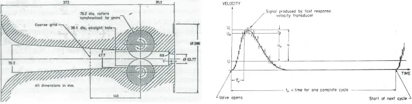
Apparatus located in the Jet Laboratory, the University of Queensland as shown in Fig. 1a produced the jet investigated. This is the same facility which was used in the earlier work reported by [5] and [6] with the exception that the jet exit diameter was halved giving a 12.77 mm diameter [22; 10]. A 200 mm disc was mounted on the nozzle to avoid directly entrainment of the fluid behind the nozzle, hence allowing the flow near the jet exit to be axisymmetric. The bulk mean jet exit velocities was kept constant as 27.6 m/s. Flow was pulsed at 5 and 10 Hz with a 1:2 ratio of time on to time off.
was then horizontally and vertically moved across the jet in small increments to determine the true jet centerline which is associated with maximum mean axial velocity.
Figure 1. (a) Pulsed jet apparatus (b) Instantaneous velocity signal of a fully pulsed jet and its basic elements
DISA 55M01 main unit with 55M11 constant temperature hot-wire anemometer (CT-HWA) adaptor was used to have velocity measurements. The hot-wire probe was a single normal wire and an overheat ratio of 1.3 was used to maintain the wire velocity sensitivity. The Kolmogorov length scale was estimated from the work of [10] giving a value of 0.124 mm. 10.16 Pm diameter Sigmond Cohn alloy 851 wire was used with the active length of 2 mm in order to give good spatial resolution. Hot-wire calibration gave a ±0.03% accuracy for the extended power-law equation improved by the look-up table method and 1.22% rms relative error of the fluctuating velocity component. To have appropriate sampling parameters for the hot-wire measurements, a sampling frequency of 1000 Hz, sample number of 50,000, and sampling time of 50 seconds were obtained from optimum digital sampling evaluation. It allowed a 0.26%, 0.45%, 1.10%, and 4.38% uncertainty of the estimated mean value, second, third, and fourth order turbulence moments; respectively.
At a fixed point near the jet exit, typical analog signal gained from the hot-wire probe was shown in Fig. 1b. The instantaneous velocity, Ui consists of the mean velocity, U and the aggregate turbulence or
fluctuating component, u. The aggregate turbulence is the sum of the pseudo and intrinsic turbulence which are represented by uP and uI, respectively. The intrinsic turbulence contains shear generated
turbulence and unsteadiness associated with the pseudo turbulence. The pseudo turbulence velocity, UP is
the phased averaged velocity at a given time delay, τP and is determined by the ensemble average of the
total instantaneous velocity over a large number of cycles at times τP from the beginning of the pulsating
cycle.
To have the velocity components of a pulsed jet associated with the instantaneous velocity, Ui, the
mean velocity, U, and the fluctuating component, u, the Reynolds decomposition holds. Estimation of the desired mean velocity can be obtained from a discrete equation over a finite time period. Throughout the present study, it holds that Uˆ = U. In the cases of spatial or time averaging, it was proved that the flow is truly steady which is shown by the results of averaging u closing to 0 (u{0), hence, an approach of a statistically stationary is valid for the intermittent turbulent flow.
2.2 Decay of inverse of the mean centerline axial velocity
¸ Existing empirical evidences [5; 14; 22; 11; 10] show that the fully pulsed jets have a linear decay rate over the pulsed dominated region (10 ≤ x/d ≤ 50).
2.3 Radial profile of the mean axial velocity
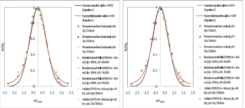
Radial profile of the mean axial velocity of the pulsed jet can be expressed in the form of a Gaussian [6; 15] and exponential [5] equation; respectively.
2 In the equations, D was equal to 0.693 [6; 15] and 0.44 [5], respectively; offering a good fit for the radial profiles.
2.4 Jet growth
For fully developed axisymmetric jets, the jet growth or jet spreading rate is indicated by the growth of the half-velocity radius, r1/2.U with x/d and can be considered to be linear. [5] and [6] formulate the jet
growth as Eq. (4) is valid both for the steady and fully pulsed jet cases by consideration that both of the jets grow linearly to the downstream regions.
2.5 Aggregate turbulence intensity
The formulation of aggregate turbulence intensity, Tu is given as
0
Subcripts “0” is added in the equation for the fluctuating component of the axial velocity and mean axial
3.Results and Discussion
3.1 Symmetric profile test and propagation of the jet
Figure 2a and b describe the results of radial symmetric profile of the mean axial velocity of the pulsed jet at the downstream positions both in the horizontal and radial direction among the recent and previous researchers [6; 10]. It is clearly seen that a high degree of the radial symmetric profiles is shown by the pulsed jets over the indicated downstream positions thus confirming the previous works by [12], [14], [11], [22], and [10]. Interestingly, it is seen that the recent and [10]’s results tend to more approach the curve fit of the exponential equation, Eq. (3) than that of the Gaussian equation, Eq. (2). With their CT-HWA, [8], [12], and [5] also produced the similar evidences. Comparing the radial profile results of a Laser-Doppler Anemometer (LDA) as in Eq. (2) [6] with those of a CT-HWA [the present researchers, 10] it is the nature of the hot-wire sensor to produce such data in the far field of the jet centerline ((r/r1/2U)
> 1.25) thus allowing a good curve fit closer with Eq. (3) rather than with Eq. (2).
Figure 2. Radial profiles of the mean axial velocity: (a) Horizontal plane (b) Vertical plane
Figure 3 demonstrates the centerline coordinates of the pulsed jet over x/d of 10, 30, 50 both in the horizontal and vertical direction. As can be seen from the figures, the centerline coordinates are relatively linear as denoted by the linear-curve fits. This is an indication that the recent pulsed jet follows a linear trajectory as it propagates further downstream. Previous researchers [i.e. 14; 22; 10] also delivered the similar evidences. For the preliminary assessment of the jet flow field, this would simply avoid the centerline determination at different axial locations x/d along the jet field.
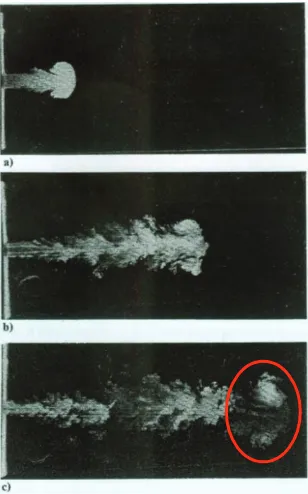
the starting vortex of [16] the present study unfortunately did not cover visualization effort. Furthermore, if the separation of the starting vortex [16] is analogous with the sudden change in the decay of the mean axial velocity [6], consequently unsymmetrical radial profiles of the mean axial velocity of the pulsed jet must result after x/d = 50. However, [14] and [10] found contradictory evidences as their pulsed jets always demonstrated the symmetrical radial profiles of the mean axial velocity even up to x/d = 60.
Figure 3. Centerline coordinates in horizontal and vertical directions
Figure 4. LIF photographs illustrating the propagation of an unsteady jet: a) t = 0.2 sec, 5d; b) t = 0.5 sec, 13 d; and c) t = 0.8 sec, 18 d.
(reproduced from Johari, Kouros et al. 1993)
3.2 Decay of inverse of the mean centerline axial velocity
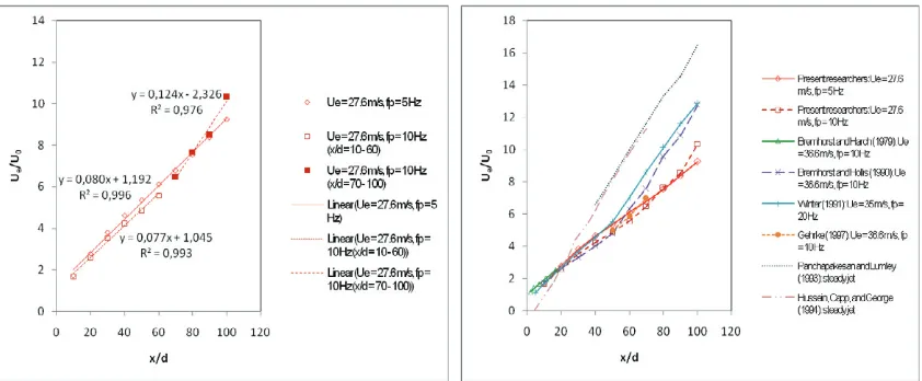
Appreciations of the decay of inverse of the mean centerline axial velocity of the pulsed and steady jets over 100 diameters downstream are shown in Figure 5a and 5b, respectively. This parameter is essential to indicate a starting point of the growth of pulsed and steady jets associated with the starting point of the decreasing mean centerline axial velocity due to little early entrainment.
From Figure 5a, it is clearly shown that the sudden change in the velocity decay heavily relies on the level of pulsing frequency. At fp = 5 Hz the velocity decay linearly grows over 100 diameters donwstream
hence resulting in no sudden change whereas at fp = 10 Hz the sudden change is seen at x/d = 60 yielding
the two distinct regions over 100 diameters downstream. Moreover, the velocity decays linearly grow over the two regions. For the recent study, the region within x/d = 10 – 60 characterizes the pulse-dominated region while the region within x/d = 70 – 100 signifies the high turbulence steady jet region. Another key point revealed is that in the pulse-dominated region the velocity decay rate at fp = 5 Hz is
slightly more rapid than that at fp = 10 Hz but the region continues to exist over 100 downstream
positions due to the endurance of the normalized periodic components (contained in one complete cycle, Figure 1b) at fp = 5 Hz. In principle, [3] explained that a cyclic compression wave (generated by the
occurs at larger x/d which in limit will switch to a steady jet associated with the sudden change in the velocity decay. Therefore, it can be concluded that the lower increase in the jet momentum at fp = 5 Hz
than that in the jet momentum at fp = 10 Hz is responsible for the more slightly rapid velocity decay than
that at fp = 10 Hz in the pulse dominated region. Furthermore, the pulse merging does not happen over
100 diameter downstream at fp = 5 Hz thus allowing the domination of the pulse-dominated region up to
further downstream due to the survival of the normalized periodic components. All of this is not to be the case for fp = 10 Hz as the complete pulse merging takes place up to x/d = 60, yielding the existence of the
two distinct regions. More importantly, as the two regions appears the pulsation imposed on the jet produces a slower velocity decay in the pulse-dominated region than that in the high turbulence steady jet counterpart.
Figure 5. Mean centerline axial velocity decay (a) Recent results (b) Comparison between the results of pulsed and steady jets
From Figure 5b, it is seen that similar evidences associated with the existence of the two regions are also demonstrated by [6] and [22] and the velocity decays are linear within the two regions, thus Eq. (1) is valid for the pulsed jet. [5] did not find the sudden change in the decay as they only performed their measurement in the first 17 diameters downstream. Yet, the present results are a continuation of [5]’s
results in the near field region. Considering the results of [10], the sudden change in the decay rate is less evident as [10]’s investigation only covered a limited axial measurement (40 < x/d < 80). Moreover, viewing the gradients of the velocity decay of steady jets [18; 15] the present researchers, [6], and [22] show the same gradients to those of the velocity decay rate of steady jets. Accordingly, the pulsed jets do turn into steady jets after the region of x/d beyond 50.
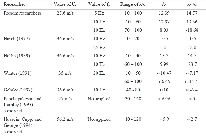
Regarding the postulation of [2] and the significance of gradient differences of the velocity decays illustrated in Figure 5b, Table 1 summarizes the decay constants in Eq. (1) for the pulsed and steady jets to be used in assessing the starting point of the jet growth (marked by the rapid entrainment) between the jets. It is seen that the values of the effective origin, x01/d for the pulsed jets in the pulse-dominated region
exponential [12; 5] or Gaussian [14; 6; 22] profiles depending on the used sensor. Besides, the level of pulsation does affect the rate of the velocity decay in the pulse-dominated region. This is clearly seen from Table 1 as the constant A1 decreases (from 12.97 to 12.39) with the lessening pulsing frequency thus
resulting in a more rapid velocity decay at fp = 5 Hz than that at fp = 10 Hz; associated with the slightly
steeper gradient at the lower pulsing frequency as seen in Figure 5a. The similar findings are also proved by [12] as seen in the table.
Comparing the two decay rates and consistent with the urgency of the effective origin of the jet therefore it can be argued that the more rapid decay rate at fp = 5 Hz in the pulse-dominated region shows
that the pulsed jet has a higher entrainment than that at fp = 10 Hz although the negative pressure gradient
at fp = 5 Hz is less than that at fp = 10 Hz owing to the less intense pulsation. However, the present
argumentation becomes complex as [1, 19, 5, 3, and 21] revealed an inverse fact with the present argumentation. The current argumentation on the other hand agrees with the findings of [8, 17, and 22] showing that an unsteady jet would become less dispersive at high pulsing frequency. To solve the ongoing debate, unfortunately the current experimental work only focuses on the pulsed jet properties along its centerline.
On top of that, the x01/d values in the far downstream region of the pulsed jets always poses negative
values as demonstrated by the steady jets [23; 14; 11; 22; 10]. This indicates that the pulsed jet has switched into a steady jet as a result of the lessening pulsation or pulse merging [6; 22]. Regarding the x01/d values of the pulsed jets in the high turbulence steady jet region which are equivalent with those of
the steady jets, some (13; 20; 18; 15] demonstrate the ‘+’ sign whereas the others [23; 14; 22; 10] show
the ‘-‘ sign. This may be due to recirculation effects of the ambient fluid in the laboratory permitting the
entrainment in the initial region, the jet centerline velocity would start to decay more early as a result of little mixing in the near field (0 < x/d < 5). Needless to say, this would shift the effective origin upstream resulting in a positive value instead of a negative one as shown by [18] and [15] but are only of the small values.
3.3 Jet growth
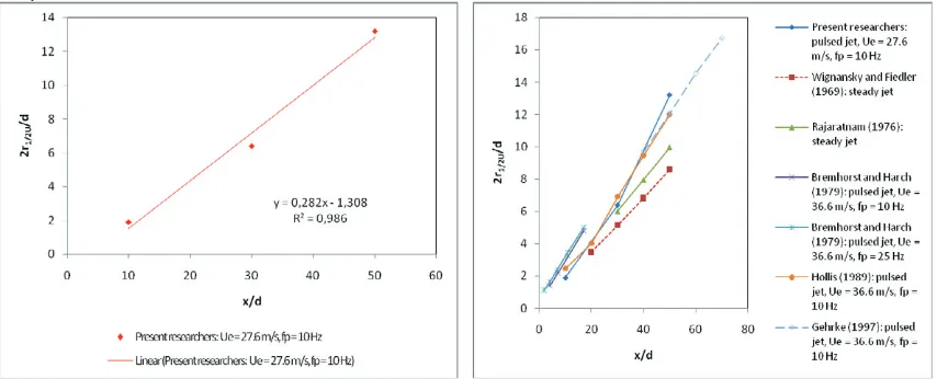
An appreciation for the growth of the pulsed jet towards further downstream is illustrated in Figure 6a. The results are evaluated from the radial profiles of normalized mean axial velocity (at fp = 10 Hz) when
the axial velocity is 0.5 U0 which corresponds to the half-value radius, r1/2.U and are plotted with a linear
curve-fit of Eq. (4). In addition, a growth comparison between the pulsed and steady jets is depicted in Figure 6b hence providing a practical consideration for their applications.
.
Figure 6. Jet growth (a) Recent results (b) Comparison between the results of pulsed and steady jets
As can be seen in Figure 6a, a linear growth of the pulsed jet is demonstrated in the pulse-dominated region which corresponds to the 50 diameters downstream. Using Eq. (4), it gives a 0.282 and -4.638 value of the A2 and x02/d, respectively. Furthermore, the present results agree with the earlier findings by
5, 14, and [10] establishing a higher growth of the pulsed jet than that of the steady jets [23; 20] despite the fragmented structural information as seen in Figure 6b. Hence, this also confirms the early findings by [8, 1, 9, 19, 3, 7, 21, 6, 4] elucidating that perturbing a jet would enhance the jet growth.
3.4 Aggregate turbulence intensity
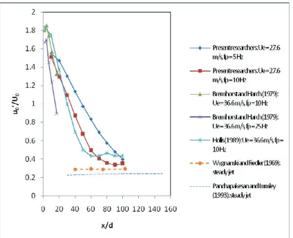
Figure 7 illustrates a comparison for the variation of the aggregate turbulence intensity, Tu along the jet centerline between the pulsed and steady jets. The recent pulsed jet was generated at Ue = 27.6 m/s
with fp = 5 and 10 Hz over 100 diameters downstream. As can be seen, the aggregate turbulence intensity
gradually decreases over 100 diameters downstream before finally reaching a relatively constant value and varies accordingly as the pulsing frequency is increased from 5 to 10 Hz. At fp = 10 Hz the aggregate
turbulence intensity decreases more rapidly along the downstream positions than that of fp = 5 Hz as a
concluded that the pulse merging at fp = 10 Hz is responsible for the the more attenuation of u0’.
Conversely, at fp = 5 Hz the pulse merging does not take place such that Tu would not reach the constant
value. Moreover, over the 100 diameters the values of the aggregate turbulence intensity at fp = 5 Hz are
higher than those at fp = 10 Hz. This indicates that at a low pulsing frequency under a constant mean exit
velocity, the jet fluids tend to be more fluctuating. To this end, this fact is consistent with the present argumentation explaining a more dispersive jet under a low pulsation and more rapid velocity decay at which produces no pulse merging at fp = 5 Hz thus resulting in the endurance of the normalized periodic
components over 100 diameters downstream.
Figure 7. Variation of the aggregate turbulence intensity along the jet centerline between the pulsed and steady jets
The patterns of the present Tu variation confirm the ones demonstrated by [5] as the pulsing frequency is increased under a constant mean exit velocity. However, [5] only studied the parameter for a limited diameter downstream (2 d x/d d 17). Moreover, the variation of Tu for the present result at fp = 10 Hz is
consistent with that of [14] but is of different magnitude due to the different nozzle diameter used. Comparing the present results with those of the steady jets, at fp = 10 Hz after the pulsed jet reaches a
constant value of Tu level at x/d > 70, the levels of Tu are bigger (reaching a value of around 35%) than those of steady jets of approximately 28% [23] and about 23.5% [18]. Therefore, the unsteady effects imposed can produce an increase in the fluctuating velocity components; even when the pulsed jet has approached a constant value of Tu level. Such evidence is also demonstrated by [8] and [24] for their unsteady jets forced by an acoustic excitation.
4.Conclusion
existence of two distinct regions. The steady jet part of the pulsed jet departs from a self-preserving steady jet having a much greater value of aggregate turbulence intensity of 35% of the mean centerline-axial velocity than that of a self-preserving steady jet. The length of pulse dominated and high turbulence steady jet region strongly depend on the varying pulsing frequency. Moreover, the velocity decay rate in the two distinct regions is found to be linear as a result of the varying pulsing frequency.
However, learning the patterns of the velocity decay rate and the existing contrary findings two crucial questions come to mind including: 1) whether the pulsed jet becomes less dispersive or not under an intense pulsation and 2) whether the pulsed jet at a certain level has a higher entrainment or not than that of a steady jet. Considering the striking issues of [2] and [16], there is no evidence of the present results which agree with the postulation and results of the former researchers explaining that the jet growth of unsteady jets should be lower than that of steady jets. Even, from the recent measurements the pulsation effects do increase the jet growth within 50 diameters downstream as compared to that of steady jet. It is demonstrated that the pulsation yields a slower velocity decay in the pulse-dominated region than that in the high turbulence steady jet region associated with the more upstream shiftness of the effective origin of the pulsed jet. Lessening the pulsation produces a more fluctuating pulsed jet associated with the augmentation of u0’ but allows a lower negative pressure gradient in the jet field as a result of a less
intense pulsation. This is the key player for the domination of unsteady effect over 100 diameters downstream thus permitting no sudden change in the velocity decay at fp = 5 Hz.
On top of that, the present results can be considered to be applied in mixing processes as the patterns of veclocity decay, the jet growth, and aggregate turbulence intensity are very clear under the varying pulsing frequency. In terms of the patterns of velocity decay, the present results can also be used to verify in turbulence models, such as k-ε model as developed by [4] to predict the decay rate. [10] explained that the failure of k-ε model [4] to predict the decay of normalized mean centerline axial velocity is due to incorrectly modeled dissipation rate. Unfortunately, such data are not provided at present with the varying mean exit velocity and pulsing frequency. [10] only provided the dissipation rate data at a limited controlled parameter: a single mean exit velocity and pulsing frequency within a limited coverage of the downstream position.
Viewing the above current progress, a continuing research therefore is of an urgent need to further explain the pulsation effects on the jet. This is essentially performed to assess the global vorticity and dissipation rate by extending the controlled parameters with an inclusion of a comprehensive radial measurement in order to explain how efficient the pulsation effects to the entrainment and spreading rate of the pulsed jet. Visualization would also be very useful to study the propagation of the starting vortex and pulse merging towards further downstream of the pulsed jet in relation to the striking findings of [16].
Acknowledgement
The first author is very grateful to Prof. Klaus Bremhorst, PhD, AM for introducing him to the field of hot-wire anemometry and for every valuable discussion during this research and to Mr. George Dick who rendered assistance in repairing hot-wire sensor. The financial support of the Technological Professional and Skill Development Project, Asian Development Bank during the present work is also very gratefully acknowledged.
References
[2] Breidenthal, R. (1986). "The Turbulent Exponential Jet." Physics of Fluid 29, no. 8: 2346-2347. [3] Bremhorst, K. (1979). "Unsteady Subsonic Turbulent Jets." Recent Developments in Theoretical and
Experimental Fluid Mechanics, Springer Verlag, Berlin: 480-500.
[4] Bremhorst, K. and L. J. W. Graham (1993). "Application of the k-H Turbulence Model to the Simulation of a Fully Pulsed Free Air Jet." Transactions of the ASME, Journal of Fluids Engineering
115: 70-74.
[5] Bremhorst, K. and W. H. Harch (1979). "Near Field Velocity Measurements in a Fully Pulsed Subsonic Air Jet." Turbulent Shear Flows I, Springer Verlag, Berlin: 37-54.
[6] Bremhorst, K. and P. G. Hollis (1990). "Velocity Field of an Axisymmetric Pulsed, Subsonic Air Jet." AIAA Journal 28, no. 12: 2043-2049.
[7] Bremhorst, K. and R. D. Watson (1981). "Velocity Field and Entrainment of a Pulsed Core Jet." Journal of Fluids Engineering 103, no. 4: 605-608.
[8] Crow, S. C. and F. H. Champagne (1971). "Orderly Structure in Jet Turbulence." Journal of Fluid Mechanics 48, part 3: 547-591.
[9] Curtet, R. M. and J. P. Girard (1973). Visualisation of a Pulsating Jet. Proceedings of the ASME Symposium on the Fluid Mechanics of Mixing, Atlanta, the United States of America.
[10]Gehrke, P. J. (1997). The Turbulent Kinetic Energy Balance of a Fully Pulsed Axisymmetric Jet. PhD Thesis, Department of Mechanical Engineering. Brisbane, The University of Queensland, Australia: 378 pages.
[11]Graham, L. J. W. (1991). Development of Experimental and Computational Techniques for Investigation of a Heated Pulsed Air Jet. PhD Thesis, Department of Mechanical Engineering. Brisbane, The University of Queensland, Australia: 257 pages.
[12]Harch, W. H. (1977). Noise and Flow Measurements in a Pulsed Jet. PhD Thesis, Department of Mechanical Engineering. Brisbane, The University of Queensland, Australia.
[13]Hinze, J. O. and B. G. Van der Heggezijnen (1949). "Transfer of Heat and Matter in Turbulent Mixing Zone of Axially Symmetrical Jet." Applied Science Research A1, no. 5-6: 435-461.
[14]Hollis, P. G. (1989). Velocity Field Investigation of A Fully Pulsed Air Jet with A Laser Doppler Anemometer. PhD Thesis, Department of Mechanical Engineering. Brisbane, The University of Queensland, Australia: 371 pages.
[15]Hussein, J. H., S. P. Capp, William K. George (1994). "Velocity Measurements in a High-Reynolds-Number-Momentum-Conserving, Axisymmetric, Turbulent Jet." Journal of Fluid Mechanics 258: 31-75.
[16]Johari, H., H. Kouros, R. Medina (1993). "Spreading Rate of an Unsteady Turbulent Jet." AIAA Journal 31, no. 8: 1524-1526.
[17]Lovett, J. A. and S. R. Turns (1990). "Experiments on Axisymmetric Pulsed Turbulent Jet Flames." AIAA Journal 28, no. 1: 38-46.
[18]Panchapakesan, N. R. and J. L. Lumley (1993). "Turbulence Measurements in Axisymmetric Jets of Air and Helium, Part I: Air Jet." Journal of Fluid Mechanics 246: 197-223.
[19]Platzer, M. F., J. M. Simmons, K. Bremhorst (1978). "Entrainment Characteristics of Unsteady Subsonic Jets." AIAA Journal 16, no. 3: 282-284.
[20]Rajaratnam, N. (1976). Turbulent Jets. Amsterdam, Elsevier Scientific Publishing Company, The Netherlands.
[21]Tanaka, Y. (1984). "On the Structure of Pulse Jet." Bulletin of JSME 27, no. 230: 1667-1674. [22]Winter, A. R. (1991). A Laser Doppler Anemometer Investigation into Fully Pulsed Jet Flows with
an Examination of Velocity Bias Error. PhD Thesis, Department of Mechanical Engineering. Brisbane, The University of Queensland, Australia.