Black was right:
Price is within a factor 2 of Value
J. P. Bouchaud, S. Ciliberti, Y. Lempérière,
A. Majewski, P. Seager & K. Sin Ronia
Capital Fund Management,
23 rue de l’Université, 75007 Paris, France
[email protected].
November 21, 2017
Abstract
We provide further evidence that markets trend on the medium term (months) and mean-revert on the long term (several years). Our results bolster Black’s intuition that prices tend to be off roughly by a factor of 2, and take years to equilibrate. The story behind these results fits well with the existence of two types of behaviour in financial markets: “chartists”, who act as trend followers, and “fundamentalists”, who set in when the price is clearly out of line. Mean-reversion is a self-correcting mechanism, tempering (albeit only weakly) the exuberance of financial markets.
Keywords: Trend following, Mean-reversion, Market Anomalies, Be-havioral biases.
1
Introduction
In his remarkably insightful 1986 piece called “Noise”, Fisher Black famously wrote [1]: An efficient market is one in which price is within a factor 2 of value, i.e. the price is more than half of value and less than twice value. He went on saying: The factor of 2 is arbitrary, of course. Intuitively, though, it seems reasonable to me, in the light of sources of uncertainty about value and the strength of the forces tending to cause price to return to value. By this definition, I think almost all markets are efficient almost all of the time.
As far as we are concerned, we always believed that Black was essentially right, precisely for the argument he sketched: humans are pretty much clueless about the “fundamental” value of anything traded on markets, except perhaps in relative terms.1
The myth that “informed” traders step in and arbitrage away any small discrepancies between value and prices does not make much sense. The wisdom of crowds is too easily distracted by trends and panic [2, 3, 4]. In Black’s view (see also [5, 6]), prices evolve pretty much unbridled in response to uninformed supply and demand flows, until the difference with value is strong enough for some mean-reversion forces to drive prices back to more reasonable levels. If Black’s uncertainty band∆ was – say –0.1%, the efficient
1As noted by O. Wilde, people know the price of everything and the value of nothing.
market theory (EMT) would be a very accurate representation of reality for most purposes. But if ∆ = 50% or so, as Black imagined, EMT would only make sense on time scale longer than the mean-reversion timeTMR, the order of
magnitude of which is set byσ√TMR∼∆. For stock indices withσ∼20%/year,
one findsTMR∼6 years.
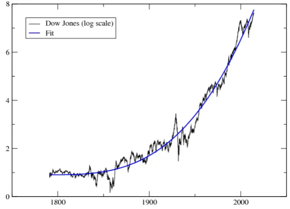
Figure 1: Dow Jones Index (in log scale) since 1791, together with a non-linear long term trend, here a simple cubic fit∝(t−t0)3witht0= 1791. This suggests
that the return of the stock market actually increases with time.
The dynamics of prices within Black’s uncertainty band is in fact not random but exhibits trends: in the absence of strong fundamental anchoring forces, investors tend to under-react to news and/or take cues from past price changes themselves [7, 4, 8, 9, 10]. This induces positive autocorrelation of returns that have been documented in virtually all financial markets – see e.g. [11, 12] and refs. therein. The picture that emerges, and that we test in the present study, is therefore the following: market returns are positively correlated on time scales
≪TMR and negatively correlated on long time scales∼TMR, before eventually
following the (very) long term fate of fundamental value – presumably a biased geometric random walk with a non-stationary drift (see Fig. 1). We test this idea on a large set of instruments: indexes, bonds, FX and commodity futures since 1960 (using daily data) and spot prices since 1800 (using monthly data). Our results confirm, and make more precise, Black’s intuition. We find in particular that mean-reversion forces start cancelling trend following forces after a time around 2 years, and mean-reversion appears to peak for channel widths ∆ on the order of50to100%, which corresponds to Black’s “factor 2”.
country start
USA 1791
Australia 1875
Canada 1914
Germany 1870
Switzerland 1914
Japan 1914
United Kingdom 1693
Table 1: Starting date of the spot index monthly time-series for each country.
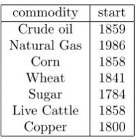
commodity start Crude oil 1859 Natural Gas 1986
Corn 1858
Wheat 1841
Sugar 1784
Live Cattle 1858
Copper 1800
Table 2: Starting date of the spot price for each commodity.
2
Data
We will use two sources of data, already exploited in our previous work on long term trend following [12]: daily data on futures contracts since 1960 and monthly data on spot contracts since 1800. The detailed description of the data can be found in [12]. In a nutshell, our futures pool contains seven commodity contracts (crude oil, natural gas, corn, wheat, sugar, live cattle and copper), seven ten-year bond contracts and seven stock index contracts (corresponding to Australia, Canada, Germany, Japan, Switzerland, the United Kingdom and the United States) and the six corresponding currency contracts. The spot contracts include the same commodities and stock indexes (with starting dates given in Tables 1, 2), bond prices since 1918 and currencies since 1973. We have actually checked that all the results shown below hold on an extended data set, where we use all contracts at our disposal. The data used in the current paper is from Global Financial Data (GFD).
3
Predictability curves over different time
hori-zons
3.1
From trends to mean-reversion
scaleT is defined as:
µt:=
1
T log
p(t)
p(t−T)
. (1)
For each contract and time t, we associate a point (x, y) where x is the de-trended past return on scale τ< and y the de-trended future return on scale
τ>:
x:= logp(t)−logp(t−τ<)−µtτ<; y:= logp(t+τ>)−logp(t)−µtτ>. (2) Note that the future return is de-trended in a causal way, i.e. no future informa-tion is used here (otherwise mean-reversion would be trivial). For convenience, bothxandyare normalised such that their variance is unity. We chooseT = 20 years and consider both:
• Spot pricesmonthlydata, extending back 200 years, withτ<= 5,10,15,20,25,30,40,50 and60months for backward looking horizons and chooseτ> =τ</5.
• Futures contractsdailydata, extending back to 1960, withτ< = 10,20,40,80,
160,320,480,640,960 and 1280 days for backward looking horizons and choose againτ> =τ</5.
In the following, we want to study how past returns on a variety of time scales from 10 days to five years predict future returns over two days to one year (respectively). The choice τ> = τ</5 is not critical to our conclusion, as we could have chosen τ> = aτ< with a ≤ 1 with similar results. Remarkably, futures and spot data lead to the same overall conclusions.
We group all contracts in two pools: one with futures and one with spots. For each each pool we group points(x, y)in sub-pools associated with different
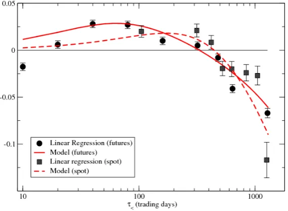
τ<. Then we fit linear regression in each sub-pool, removing outliers (i.e. |x|>4 or|y|>4). The slopes of this regression are shown in Fig. 2. For short lagsτ<<∼ 2 years, the slope is positive, compatible with the well known trend following effect (τ< = 5 months exactly recovers the results of [12] for spot prices). But for longer lags, a clear mean-reversion effect is observed, with a negative slope increasing (in absolute value) with time horizon. The pattern is very similar for spot and futures data, although in the latter case some evidence for short term mean-reversion when τ< = 10 days can be detected. The appearance of long-term reversion on multi-year time scales was first evidenced by Poterba and Summers in the case of stock indices [6].
3.2
A simple model
It is insightful to compare the behaviour of the regression slope shown in Fig. 2 with a simple model. Assume that the de-trended log-price π(t) evolves as a mean-reverting Ornstein-Uhlenbeck process driven by a positively correlated (trending) noiseη, to wit:
dπ(t) where κ−1 is the mean-reversion time, γ−1 the trend correlation time andg a
parameter measuring the strength of the trend. One can compute analytically the regression slopes(τ<, τ>)of future returns on scaleτ> as a function of the past returns on scaleτ<. After some manipulations (see Appendix), one finds:
s(τ<, τ>) =
C(τ<) +C(τ>)−C(τ<+τ>)−1
2p
(1−C(τ<))(1−C(τ>))
(4)
where the autocorrelation functionC of the processπis defined as:
C(u) := 1
simplicity of the model, the qualitative agreement is quite remarkable. Although the value of the parametersg, κand γ are not determined with high accuracy, their order of magnitude is reasonable. Note that by construction our stylized model is unable to account for any short-term mean-reversion, and significant discrepancies are indeed observed forτ<<∼20days for which the slopesbecomes negative.
If the model defined by Equation (3) is taken seriously, the mean square fluctuations of the log-price around its equilibrium value is easily computed to be:
hπ2i=σ2(1 +g), (6) which we define as the square of the width of Black’s uncertainty band, ∆2.
model, one can infer the value of σ from market data. Taking a typical daily volatility of 1%, one findsσ2 = 0.2and ∆≈0.5for futures data and σ2= 0.1
and ∆ ≈ 0.35 – corresponding to prices erring by a factor ∼ 1.5 from their “reference” value, much as Black argued [1]. While the precise value of∆should not be taken too seriously, we find our results quite suggestive.
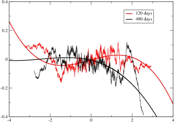
Figure 3: Plot of y (de-trended future return on scaleτ> =τ</5) vs. x (de-trended past return on scaleτ<) for futures daily data, andτ< = 120business days (red lines) and τ< = 480 business days (black lines). We show both a running average through 200 consecutive points, and a cubic fit of the raw data (excluding points beyond 4-σ). The change of slope sign as τ< increases, and the presence of non-linear effects, are clearly suggested by these plots.
3.3
Non-linear effects?
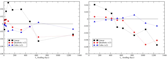
A closer look at the plot (x, y) however reveals significant departure from a simple linear behaviour – see Fig. 3. One expects trend effects to weaken as the absolute value of past returns increases, as indeed reported in [12]. We have therefore attempted a cubic polynomial regression, devised to capture both potential asymmetries between positive and negative returns, and saturation or even inversion effects for large returns. The linear, quadratic and cubic coefficients of the fit are also shown in Fig. 4. The linear coefficient of the fit behaves very similarly to the slope of the simple linear regression, as expected. Our conclusion on the change of sign of the slope aroundτ<= 2years is therefore robust. The quadratic term, on the other hand, is positive for short lags but becomes negative at longer lags, for both data sets. The cubic term appears to be negative for all time scales in the case of futures, but this conclusion is less clear-cut for spot data.
term, on the other hand, suggests that large moves (in absolute value) tend to mean-revert, as expected, even on short time scales where trend is dominant for small moves. Taking these non-linearities into account however does not affect much the time scale for which the linear coefficient vanishes, i.e. roughly two years.
Figure 4: Cubic fit parameters as a function of past horizon τ< for (left) fu-tures daily data and (right) spot monthly data. Note that the linear coefficient changes sign around τ< = 2years (500 trading days), as is found for the slope of the simple linear regression (see Fig. 2).
4
Conclusion
In this paper, we have provided some further evidence that markets trend on the medium term (months) and mean-revert on the long term (several years). This dovetails with Black’s intuition that prices tend to be off by a factor of two: it takes roughly six years for the price of an asset with 20 % annual volatility to vary by 50 %.
Such a long time scale is another nail in the coffin of efficient market theory: as anticipated by Summers and others [5, 6], it is not because returns are only weakly correlated on short time scales that prices efficiently reflect value. The story behind our results, on the other hand, fits well with a series of previous models [13, 14, 15, 16, 17], which postulate the presence of two types of agents in financial markets: “chartists”, who act as trend followers, and “fundamen-talists”, who set in when the price is clearly out of whack. Mean-reversion is a self-correcting mechanism, tempering (albeit only weakly) the exuberance of financial markets.
From a very practical point of view, our results suggest that universal trend following strategies should be supplemented by universal price-based “value” strategies that mean-revert on long term returns.2
As is well known, trend following strategies offer an hedge against market drawdowns (see e.g. [19]); value strategies offer a hedge against over-exploited trends. As a consequence, we find that mixing both strategies significantly improves the profitability of the resulting portfolios.
2Value strategies based on more fundamental (but less universal) indicators have been
Acknowledgments: We thank L. Duchayne, A. Rej and M. Potters for useful insights, and A. Breedt for comments.
Appendix
The dynamics of process πis given by Eq. (3). Using variation of parameters we can write
For larget,π(t)admits stationary distribution with zero mean. Lets compute covariance of the process:
and the variance of the process is equal σ2(1 +g). Then, it is straightforward
to obtain the slope of linear regression ofπ(t+τ>)−π(t)onπ(t)−π(t−τ<) from the covariance of π(t), with the result given in the main text.
References
[1] F. Black,Noise. Journal of Finance, 41 529-543 (1986).
[2] C. MacKay, Memoirs of Extraordinary Delusions and the Madness of Crowds. (1852), reprinted by L. C. Page, Boston (1932).
[4] J. DeLong, A. Bradford, A. Shleifer, L. H. Summers, and R. J. Waldmann,
Positive feedback investment strategies and destabilizing rational specula-tion. Journal of Finance 45:379-95 (1990).
[5] L. Summers,Does the Stock market rationally reflect fundamental values?. Journal of Finance, XLI, 591 (1986).
[6] J. M. Poterba, L. Summers,Mean reversion in stock prices: Evidence and implications. Journal of Financial Economics, 22(1), 27-59 (1988).
[7] W. de Bondt, R. H. Thaler, Does the stock market overreact?. Journal of Finance 42, 557-581 (1985).
[8] H. Hong, J. Stein, A Unified Theory of Underreaction, Momentum Trad-ing, and Overreaction in Asset Markets. Journal of Finance 54, 2143-2184 (1999).
[9] D. Kent, D. Hirshleifer, A. Subrahmanyam, Investor Psychology and Se-curity Market Under- and Over-reactions. Journal of Finance, 53, 1839-85 (1998).
[10] J.-P. Bouchaud, Ph. Krueger, A. Landier, D. Thesmar,Sticky Expectations and the Profitability Anomaly, https://ssrn.com/abstract=2742730
[11] M. Covel, Trend Following: How to Make a Fortune in Bull, Bear and Black Swan Markets. Wiley (2017).
[12] Y. Lempérière, C. Deremble, P. Seager, P., M. Potters & J. P. Bouchaud,
Two Centuries of Trend Following. Journal of Investment Strategies 3, 41-61 (2014).
[13] R. Day, W. Huang, Bulls, bears and market sheep. Journal of Economic Behavior and Organization, 14, 299-329, (1990).
[14] T. Lux, M. Marchesi, Volatility clustering in financial markets: a micro-simulation of interacting agents. Int. J. Theor. Appl. Finance 3, 675 (2000).
[15] I. Giardina, J.-P. Bouchaud, Bubbles, crashes and intermittency in agent based market models, Eur. Phys. J. B 31, 421 (2003).
[16] C. H. Hommes, Heterogeneous agent models in economics and finance. Handbook of computational economics, 2, 1109-1186, (2006).
[17] C. Chiarella, X. Z. He, & C. Hommes, A dynamic analysis of moving av-erage rules. Journal of Economic Dynamics and Control, 30(9), 1729-1753 (2006).
[18] C. S. Asness, T. J. Moskowitz, L. H. Pedersen, Value and momentum ev-erywhere. The Journal of Finance, 68(3), 929-985 (2013).
