CHANGE ANALYSIS OF LASER SCANS OF LABORATORY ROCK SLOPES SUBJECT TO
WAVE ATTACK TESTING
Yueqian Shena,b, Roderik Lindenberghb, Bas Hoflandc, Roy Kramerc
a. School of Earth Science and Engineering, Hohai University, No.1, Xikang Road, Nanjing 210098, China – [email protected]
b. Department of Geoscience and Remote Sensing, Delft University of Technology, Stevinweg 1, 2628 CN, Delft, The Netherlands – [email protected]
c. Department of Hydraulic Engineering, Delft University of Technology, Stevinweg 1, 2628 CN, Delft, The Netherlands – [email protected], [email protected]
Commission II, WG II/10
KEY WORDS: Coastal Engineering, TLS, Change Analysis, Water Flume, Wave Attack, Breakwater
ABSTRACT:
For better understanding how coastal structures with gentle slopes behave during high energy events, a wave attack experiment representing a storm of 3000 waves was performed in a flume facility. Two setups with different steepness of slope were compared under the same conditions. In order to quantify changes in the rock slopes after the wave attack, a terrestrial laser scanner was used to obtain 3D coordinates of the rock surface before and after each experiment. Next, through a series of processing steps, the point clouds were converted to a suitable 2D raster for change analysis. This allowed to estimate detailed and quantitative change information. The results indicate that the area around the artificial coast line, defined as the intersection between sloped surface and wave surface, is most strongly affected by wave attacks. As the distances from the sloped surface to the waves are shorter, changes for the mildly sloped surface, slope 1 (1:10), are distributed over a larger area compared to the changes for the more steeply sloped surface, slope 2 (1:5). The results of this experiment show that terrestrial laser scanning is an effective and feasible method for change analysis of rock slopes in a laboratory setting. Most striking results from a process point of view is that the transport direction of the rocks change between the two different slopes: from seaward transport for the steeper slope to landward transport for the milder slope.
1. INTRODUCTION
Due to climate change with its associated rising sea level, tidal effects and expected increases in the intensity and frequency of storms the risks of coastal erosion are expected to increase (Nicholson-Cole, 2005). Different types and configurations of structure have been used to protect our coasts against erosion, most commonly consisting of piled rocks. With rapid erosion of coastal structures, the demand for natural rock has increased all over the world, especially in the Netherlands and other low lying countries with significant coast length. An important question is what configuration of rocks provide optimal protection in a given wave climate (Van Der Meer, 1988). The stability of rock slopes consisting of loose rocks under wave attack has been investigated before, (Van Der Meer, 1988). An extensive research of laboratory studies employing random waves was performed on the stability of so-called riprap slopes (Thompson and Shuttler, 1975). The stability of rock slopes in the range from 1:1.5 to 1:4 were tested by performing 250 tests, the results presented the probability distribution of run-up on rock slopes (Van der Meer and Stam, 1992). These older tests typically use a mechanic profiler to obtain ~10 transects of the profile development, and thereby don’t capture the full redistribution of bed material. In later research, the rates and mechanisms of changes in rock slopes were also examined by distinct element computer modelling using field and laboratory data (Allison and Kimber, 1998). A detailed structural analysis of rock slope relief was demonstrated using a digital elevation model (Jaboyedoff et al., 2007). The measurement technique of 3D Digital Stereo Photography was applied to assess the damage to rubble mound structures (Hofland et al., 2013). The damage to 3D rubble mound structures was also described and
sounder data to quantify damage to a breakwater (Tulsi, 2016). Nevertheless, little literature discusses applications of terrestrial laser scanning in coastal engineering. Here, we propose to measure the rock surfaces at a lab scale of ~0.8 m x 40 m using terrestrial laser scanning to detect changes by comparing repeated point clouds. The aim of the research presented here is to evaluate the influence on the different slopes caused by wave attack and address the application of TLS in coastal engineering at lab conditions.
In our study, a test for evaluating the impact of waves on two rock slopes of different steepness has been carried out. The flume is designed for modelling coastal structures and to assess their safety against wave attack, storm surges and flooding. In this experiment, two mild slopes (1:10 and 1:5) are tested under set wave conditions to determine their stability. The stability on its turn is derived from the profile change after a JONSWAP wave spectrum (Hasselmann et al., 1973). The spectrum represents a typical Dutch storm consisting of 3000 waves. The wave attack was simulated by a wave generator (Dodaran et al. 2015). The tests are done in the water flume of Delft University of Technology and the flume has a length of 40m, a width of 0.8m and a height of 0.9m. The stones used on the slope have a median nominal diameter of 16.2 mm, and are placed at a layer thickness of two times the nominal diameter (i.e. ~32 mm). A surface view of the stones is shown in Figure 1.
Figure 1. Surface view of the stones
2. MATERIALS AND METHODS
In this section, the materials, instruments and setup used in the wave attack experiment are described as well as the methodology for processing the point clouds. First, the wave attack experiment and its observation using laser scanning is discussed in section 2.1. Detailed processing of the point clouds is discussed in section 3.2.
2.1 Experiment description and scan data acquisition 2.1.1 Water flume and wave experiment
In our experiment, two types of slopes, 1:10 and 1:5, were tested under set wave conditions to determine their stability. The stability on its turn is derived from the profile change after a wave series that present a Dutch storm event including 3000 waves. Since the experiment was conducted in a laboratory, artificial lighting from the ceiling was present. A special wooden construction, see figure 2, left, was made to mount the terrestrial laser scanner directly above the stone slope. In order to simulate real coastal conditions, the wave surface did not cover the entire slope, see figure 3, where the oblique surfaces surrounded by solid lines are rock slope 1 (1:10) and rock slope 2 (1:5) respectively, while the blue dashed line represents the wave surface. The red dashed line indicates the intersection line (coast line) between still wave level and the two rock slopes respectively. In addition, figure 3 shows the relative position of TLS, rock slopes and water flume. Note that the different scans were made when there was no water in the flume, i.e. water was drained after each experiment. The process of draining is assumed to have no influence on the bed level.
Figure 2. Left. Special wooden construction for mounting the laser scanner above the flume. Right. Scanner view of the scene.
The along flume direction is denoted Y in this work, and the across flume direction X, in the local slope coordinate system.
2.1.2 Influence of wet stones on point cloud quality
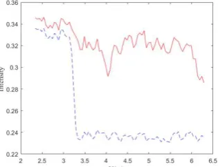
The experiment was performed from 14 August to 28 September 2016. Scanning was carried out before and after the wave testing. After the wave tests, always two scans were obtained, one was obtained just after the flume water got drained, therefore the stones on the bed were still wet. The second one was obtained after the stones had dried up. Laser scanners not only provide information about the 3D location of object surfaces but also store the amount of reflected energy as an intensity value. Often a color camera is integrated to obtain true RGB colors of the object surface. For interpreting the influence of moisture on the quality of the point clouds, a figure showing the intensity profile along the flume direction is plotted, as shown in figure 4: the red solid line represents the intensity profile for a dry point cloud while the blue dashed line represents the intensity profile for the corresponding wet point cloud. It is apparently that a sudden jump of intensity occurs in the wet point cloud. The position of sudden change is located near the intersection line: on the left of that area the stones are always dry. Therefore, the influence of moisture on the intensity of point cloud is easily obtained by comparing the intensity difference on the right of intersection area. This experiment shows that the wetness of the rocks has a serious negative effect on the intensity. A lower intensity also implies a lower Signal to Noise ratio, which will in turn affect the precision of individual points. In order to avoid the influence of moisture on the quality of the point clouds, in the following analysis scans are used that were obtained after the rocks turned dry.
Figure 4. Intensity profiles along the Y axis, i.e. the along flume direction. The red solid line is the profile of the dry point cloud; the blue dashed line is the profile for the corresponding wet point cloud. A intensity value at a given Y location is obtained by averaging intensities for all corresponding X values.
2.1.2 Scan settings
A Leica C10 Scan Station scanner (Leica, Heerbrugg, Switzerland) was used for this experiment. This scanner, with an effective range of 300 m at 90% reflectively, exploits a time-of-flight principle for measuring the range between scanner and object. The reported accuracy of a single measurement is 6 mm (one sigma) in position and 4mm (one sigma) in depth at ranges up to 50 m (Geosystems, 2012). We interpret the positional accuracy as the pointing angle accuracy, and the depth accuracy as the range accuracy. Two scans were made for each epoch. The first scan was made at minimum resolution corresponding to 0.2 m horizontal and vertical spacing at a range of 100 m (Mohd Azwan et al., 2013), at full field of view. The second scan was high-resolution corresponding to 0.02 m horizontal and vertical spacing at a
the point density of the processed scans is 288000 2
/
Table 1 Number of points of the processed scans
Slope type Number of Points favorable incidence angles. During the experiment, also point clouds were obtained from an opposite position, with more favorable measurement geometry, but these scans could not be used in this analysis as the measurement scene was disturbed by an external agent. In order to guarantee accurate registration, three targets were positioned along the water flume frame. The positions of scanner, targets and slope are shown in the scanner view of the experiment scene, see the right figure 2 (taken from the scanner centre). two epochs are expected to be in a common coordinate system before detecting changes. Registration aligns and combines multiple data into a single set of range data. Therefore, registration of the two point clouds from the two epochs is a vital pre-processing step.
In our study, the Tie Control Point method (TCP) is employed for the registration of various scans. Targets of special material manufactured by Leica are used and their centroid is extracted with high accuracy by the scanner itself. Thereby, the Leica Cyclone software could provide an automatic registration method based on TCP, (Shen et al. 2017). Considering the characteristics of the water flume with a long length compared to its width, it is difficult to place targets with a strong geometry. However, due to the high accuracy of the target centre extraction algorithm by Leica Cyclone, a high precision least squares registration could be performed: the errors for the three targets at two slopes are less than or equal to 1 mm.
2.2.2 Coordinate transformation
To obtain the change information in a more intuitive way, a so-called slope coordinate system is introduced. The initial coordinates, X' ,Y' and Z' values obtained by TLS, are
determined by the location of the TLS (i.e., distance of TLS to the object and its orientation angle), see figure 3. However, the expected displacement, perpendicular or along the slope does not correspond to the TLS coordinate system (O X Y Z'- ' ' ').
Principle component analysis (PCA) is used to estimate a 3D transformation from the TLS coordinate system to the slope coordinate system (Van Goor et al., 2011). PCA estimates the consecutive orthogonal directions in the point cloud of maximal variation. (Jolliffe 2014). The first PCA component corresponds to the direction in the point cloud with the largest variance, the along slope direction. The second component corresponds to the across slope direction, while the third component points in the direction normal to the sloped plane.
Note that the point cloud used for estimating the eigenvectors is in fact the union of two point clouds after registration: one is acquired before the wave attack experiment and the other is acquired after the wave attack experiment.
2.2.3 Raster image creation
After transformation, the slope is parallel toXOY. To simplify segmentation and change analysis in the direction perpendicular to the slope plane, a 2.5D approach was employed, core idea of which is to lattice the point cloud of the slope into a regular grid with 2D support. The approach reduces the 3D point cloud to a 2D domain by creating a 2D raster image. The attribute of each pixel in the 2D raster image is the
Zvalue in the slope coordinate system which is estimated by averaging theZcoordinate values of all points within the raster cell. The raster image’s resolution is determined by the pixel size and its bounding box is calculated from the maximum and minimum coordinates of the point clouds. As a consequence, the accuracy of detecting changes is constrained by the pixel size. The choice of pixel size is determined by considering storage, computational efficiency, required accuracy and practical necessity.
2.2.4 Change detection from raster image
Once the two point clouds are in the same slope coordinate system, a raster grid ofm rows in theY direction and n
columns in the X direction is built in the slope plane coordinates. In this work, the pixel size is first set as the triple average diameter of the rocks which is approximately 0.05 m. This value is chosen as it is ~3x the average stone diameter, and therefore partly smooths out edge effects and the like. This ensures that the pattern of displacement is analyzed rather than the movement of individual rocks. The next step is to calculate the attribute, here the average Z value, of each pixel in the raster structure. For a given pixel cell, all points in the corresponding area are determined and the average the of the Z values of all points in the pixel is stored as the attribute value of this pixel (ZA i j , i1,2, m j,1,2, n ). Then, the profile of change
along the slope length (Y direction) is defined and computed by averaging all pixel values in the same row, following
respectively, in the raster image. The change profile along the X axis is determined in a similar way.
3. RESULTS
Before extracting changes from the rock slope, we scanned, registered, and transformed the coordinates of the point clouds from two epochs as discussed above.
3.1 Detected changes
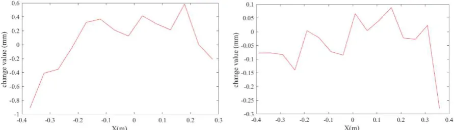
The red lines in figure 5 show the change profile of the two slopes (1:10 and 1:5) along the Y axis. The maximum and minimum values of change of slope 2 (1:5) are about 1.5 mm and -2.2 mm respectively. The maximum and minimum change of slope 1 (1:10) are more significant with values of about 6.0 mm and -5.0 mm. These two figures indicate that most change happened at the area around the coast line. A possible explanation is that this is the location where runup and rundown velocities are highest; In the other areas, changes are relatively small with an average value is around 0 mm. The changes at slope 1 (1:10) more frequently fluctuate compared to those of slope 2 (1:5). The difference between the two slopes corresponds well to the practical situation: in figure 3, it is noticeable that the points in rock slope 1 (1:10) are always more close to the wave surface compared to the points in rock slope 2 (1:5), which indicates that the amount of change is related to the distance to the waves. Note that in Figure 5, right, a shift appears to occur in the Y direction from the red line (5 cm grid) to the blue line (1.6 cm grid). As both profiles represent the same signal but sampled at different intervals, we interpret this shift as caused by this sampling difference.
Figure 5. Change profile along the Y axis (left for slope 1 and right for slope 2), i.e. the along flume direction. A change value at a given Y location is obtained by averaging all changes for the corresponding X values. The red line represents the slope change profile
for the entire flume obtained with a pixel size of 0.05 m. The blue line is the change profile restricted for the ROI obatined with a smaller pixel size of 0.016 m.
Figure 6. Change profile along the X axis (left for slope 1 and right for slope 2), i.e. the across flume direction. A change value at a given X location, is obtained by averaging all changes for the corresponding Y values. It is assumed that these profiles are affected by
some leakage that took place at the side of the flume.
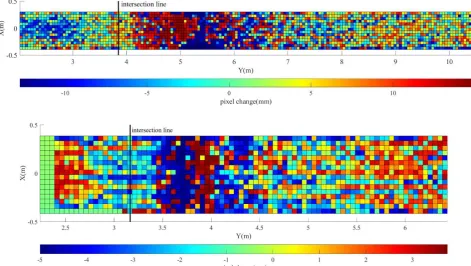
For a detailed interpretation of the change, we plotted the full raster image colored by the pixel change, see figure 7. The intersection line, or coast line, between the still water level and the slope is depicted in the figures as well. The distance of these coast lines for these two slopes to the origin are about 3.85m and 3.17m respectively, in the slope coordinate system. The greatest pixel change of slope 1 happened between [4,6.5] m in the Y direction while the greatest pixel change of slope 2 happened between [3.5 4.5] m in the identical direction. The pixel change values of the two slopes are in the ranges [-12.77 14.83] mm and [-5.01 3.75] mm, respectively. (within the symbol [ ], the left value represent the minimum value and the right value the maximum value). The mean pixel change values of the two slopes are 0.04mm and -0.04 mm. Here we conclude that the amount of change for mild slope 1 is a factor 2 to 3 times higher as for the steeper slope 2, which can again be explained by the higher proximity of the waves to the rocks for the mild slopes. The total volume changes on the left and right of the coast line in slope 1 are -191.36 mm3 and 454.29 mm3
respectively, and the mean volume change for each pixel on the left and right of the coast line in slope 1 are -0.37 3
mm and 0.25 3
mm . For slope 2, the corresponding total volume change value for slope 2 are 5.1 3
mm and -144.2 3
mm respectively, and the mean volume change value for each pixel is 0.017mm3
and -0.015 3
mm . Note that the direction of transport changes between the two tested slopes. Indeed, for the steeper 1:5 slope, transport is mostly seaward, that is towards the positive Y direction, while for the less steep 1:10 slope, transport is in the opposite direction, the negative Y direction.
The way the laser scanner is operating from a fixed position,
compare Figures 3, will inevitably result in variations in quality and point density of the acquired point cloud in notably the along flume direction (Soudarissanane et al., 2011). Therefore, the number of points in each pixel is determined. Figure 8 shows the raster image colored by the number of points per pixel for Slope 1. As the scans were made from the top side of the slope, number of points per pixel is higher close to the scanner than it is further away. At larger distances to the scanner, the number of points per pixel is dropping dramatically. But, as the figure 2 shows, change at larger distances is very limited, therefore we conclude that the measurement geometry has little influence on the results. Another effect that should be noted is that near the edges of the flume, the number of points per pixels also drops, which is causes by the grid dimension, relative to the dimensions of the flume, often resulting in incomplete pixels.
deeper` between the rocks close to the scanner than at larger
distances. Therefore, more variation with respect to the average bed level is expected at shorter distances to the scanner.
Figure 7. Raster image colored by pixel change for both slopes ( top for slope 1 and bottom for slope 2). A pixel change value is obtained by differencing the mean of the Z values for the corresponding pixel in two epochs. Negative pixel change values indicate
that erosion happened in a pixel while positive pixel change value indicates. Note that the area covered by Slope 1 is longer as the slope grade is more gentle and therefore covers a longer area.
Figure 8. Raster image of Slope 1, colored by number of points in each pixel . The attribute of each pixel is determined by counting the number of points in that pixel. The closer the distance to the scanner, the higher the number of points per pixel.
Figure 9. Raster image for Slope 1 colored by the standard deviation per pixel. A pixel standard deviation is obtained by computing the standard deviation of all Z values in the pixel.
3.2 Interest area analysis
Obviously, the change in the area near the intersection line is greater than in other areas, which indicate that this is where
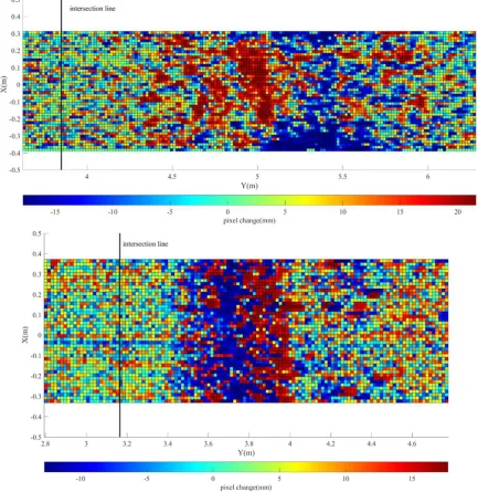
region of interest (ROI). Here, the pixel size is set at approximately the stone diameter,i.e. at a value of 0.016 m, to allow for a more detailed analysis. The raster image is built again as discussed above.
The blue line in figure 5 shows the change profile of the two ROIs (1:10 and 1:5) along the Yaxis. For the steeper Slope 2, change only has a greater fluctuation in the ROI; For milder Slope 1, the absolute change values are larger. The maximum and minimum change along theYdirection for mild Slope 1 are 6.15 mm and -5.61mm; while for Slope 2 these numbers are 1.51mm and -2.53 mm. The mean change of the two slopes in the Y direction are 0.26 mm and -0.10 mm respectively. Note that, the maximum change, minimum change and mean change of the ROIs are approximately equal to the full slope results discussed above which indicates that the pixel size has little
influence on the absolute change profile along the Y direction. Figure 10 show the pixel change of ROI belonging to the slope 1. The maximum pixel change values (maximum accretion) of the two slopes are 21.58 mm and 17.71 while the minimum pixel change values (maximum erosion) are -17.80 mm and -12.72 mm respectively Note that, compared to the pixel change value for the full area introduced in section 3.1, the absolute maximum change, minimum change and mean change values are all smaller which result from the pixel size, namely the greater the pixel size the absolute pixel change value is smaller. Obviously, if the pixel size is greater than the nominal diameter of the stone (i.e. 16.20mm), one pixel covers more than one complete stone and it causes the accretion or erosion of the current pixel averaged by the region outside the stone.
Figure 10. More detailed raster image of changes before and after the wave attack (top for slope 1 and bottom for slope 2). Pixels are colored by the change value
3.3 Validation: volume comparison
Within the test setting, in principle no stones can be lost, they
validation of the methodology, it is therefore checked if indeed the total stone bed volume stays the same, as expected. The volume change for each pixel of the two ROIs is estimated at a value of 0.068 3
mm and -0.0233 3
evident that the sum of accretion and erosion is not equal to zero. However, the absolute deviation is relatively small. Considering the registration error and edge affects, we have reasons to believe that the change analysis is reliable. The above ROI change analysis results correspond well to the entire slope change analysis.
3.4 Outlook to future work: analysis at stone level
As future work, we would recommend to study a more detailed quantitative analysis of the surface change, by incorporating single rock extraction (as marked in Figure 11). This will definitely be an interesting work from a laser scanning
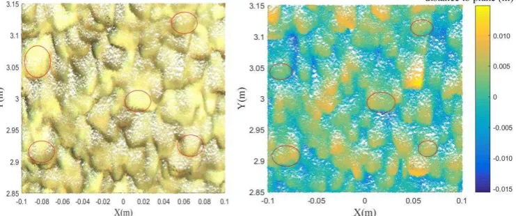
processing perspective. If it has additional value from a process point of view, is under discussion: on one hand, an analysis at single rock level may give no new information on the process, as the movement of individual rocks can be regarded as a random process. It could be argued that only by analyzing ensemble averages, as presented in this paper, the effect of the process, the motion induced by waves on a given rock slope, is becoming visible. On the other hand, the process is constrained in certain ways by gravity, wave forces and friction between rocks. Better understanding of the relative impact of those constraints could possibly be obtained by an analysis at single rock level.
Figure 11. Raw data of the stones, left colored by RGB and right colored by the distance to the slope plane. `Negative` distances up to 15 cm represent points below the slope plane; positive distances come from points above the slope plane: several single stones are
highlighted.
4. CONCLUSIONS
The applicability of using laser scanning for change analysis for rock slopes in a flume facility has been confirmed in this study. We have provided overall change estimates of two slopes under the same wave attack regime. Besides the change tendency, we also provided a detailed analysis based on a raster image analysis in the region of interest near the intersection line between the wave surface and the slope plane. The results indicate that rocks near the intersection line trends are easily changed by wave attack. In addition, the change value under the action of waves is closely related to the distance between the slope and the wave in the vertical dimension. However, the mathematical model between change values and the distance is not given. Finally, the results show that the transport directions actually swaps from seaward, for the steeper 1:5 slope, to landward, for the less steep 1:10 slope. This result is interesting for the future design of rock beds. We believe that our experiments provide important information and give guidance for researchers to apply terrestrial laser scanning in coastal engineering.
5. ACKNOWLEDGEMENTS
We would like to thank China Scholar Council (CSC) for enabling Yueqian Shen to study for one-year at the Department of Geoscience and Remote Sensing, TU Delft. We also would like to thank the Department of Hydraulic Engineering at TU Delft for providing the wave flume facility, and to acknowledge de Vries & van de Wiel (member of the DEME-Group) who supported and guided the MSc work of Roy Kramer.
REFERENCES
Allison, R. J. and O. G. Kimber, 1998. Modelling failure
mechanisms to explain rock slope change along the Isle of Purbeck coast, UK. Earth Surface Processes and Landforms, 23(8), pp.731-750.
Capra, A., E. Bertacchini, C. Castagnetti, R. Rivola and M. Dubbini, 2015. Recent approaches in geodesy and geomatics for structures monitoring. Rendiconti Lincei, 26(1), pp.53-61.
Dodaran, A. A., S. K. Park, K. H. Kim, M. E. M. Shahmirzadi and H. B. Park, 2015. Effects of Roughness and Vertical Wall Factors on Wave Overtopping in Rubble Mound Breakwaters in Busan Yacht Harbor. Journal of Ocean Engineering and Technology, 29(1), pp.62-69.
Geosystems, L., 2012. Leica ScanStation C10. Product Specifications: Heerbrugg, Switzerland.
Hasselmann, K., T. Barnett, E. Bouws, H. Carlson, D. Cartwright, K. Enke, J. Ewing, H. Gienapp, D. Hasselmann and P. Kruseman, 1973. Measurements of wind-wave growth and swell decay during the Joint North Sea Wave Project (JONSWAP), Deutches Hydrographisches Institut.
Hofland, B., E. Diamantidou, P. van Steeg and P. Meys, 2015. Wave runup and wave overtopping measurements using a laser scanner. Coastal Engineering, 106, pp.20-29.
Hofland, B., M. Disco and M. Van Gent, 2014. Damage characterization of rubble mound roundheads. Proc. CoastLab 2014, Varna, Bulgaria.
Jaboyedoff, M., R. Metzger, T. Oppikofer, R. Couture, M. Derron, J. Locat and D. Turmel, 2007. New insight techniques to analyze rock-slope relief using DEM and 3D-imaging cloud points: COLTOP-3D software. In: Rock mechanics, 1, pp. 61-68
Jolliffe, I., 2014. Principal component analysis, Wiley StatsRef: Statistics Reference Online.
Lindenbergh, R., L. Uchanski, A. Bucksch and R. Van Gosliga, 2009. Structural monitoring of tunnels using terrestrial laser scanning. Reports on Geodesy, 2(87), pp.231-238.
Mohd Azwan, A., S. Halim, M. Zulkepli, K. Albert, M. Khairulnizam and A. Anuar, 2013. Calibration and accuracy assessment of Leica scanstation C10 terrestrial laser scanner. Development in Multidimensional Spatial Data Models.
Springer Lecture Notes in Geoinformation and Cartography, pp.33-47.
Nicholson-Cole, S. A., 2005. Representing climate change futures: a critique on the use of images for visual communication. Computers, Environment and Urban Systems,
29(3), pp.255-273.
Pesci, A., G. Teza and E. Bonali, 2011. Terrestrial laser scanner resolution: Numerical simulations and experiments on spatial sampling optimization. Remote Sensing, 3(1),pp. 167-184.
Puente, I., R. Lindenbergh, H. González-Jorge and P. Arias, 2014. Terrestrial laser scanning for geometry extraction and change monitoring of rubble mound breakwaters. ISPRS Annals, 2(5), pp.289.
Puente, I., J. Sande, H. González-Jorge, E. Peña-González, E. Maciñeira, J. Martínez-Sánchez and P. Arias, 2014. Novel image analysis approach to the terrestrial LiDAR monitoring of damage in rubble mound breakwaters. Ocean Engineering, 91, pp.273-280.
Raaijmakers, T., F. Liefhebber, B. Hofland and P. Meys, 2012. Mapping of 3D-bathymetries and structures using stereophotography through an air-water-interface. Coastlab 12, pp.17-20.
Shen, Y., R. Lindenbergh and J. Wang, 2017. "Change Analysis in Structural Laser Scanning Point Clouds: The Baseline Method. Sensors, 17(1), pp.26.
Soudarissanane, S., R. Lindenbergh, M. Menenti and P. Teunissen, 2011. Scanning geometry: Influencing factor on the quality of terrestrial laser scanning points. ISPRS Journal of Photogrammetry and Remote Sensing, 66(4), pp.389-399.
Streicher, M., B. Hofland and R. Lindenbergh, 2013. Laser ranging for monitoring water waves in the new Deltares Delta Flume, ISPRS Annals, II-5/W2, pp. 271-276
Thompson, D. and R. Shuttler, 1975. Riprap design for wind wave attack. A laboratory study in random waves. Technical Report, HR Wallingford.
Tulsi, K. R., 2016. Three dimensional method for monitoring damage to dolos breakwaters, PhD dissertation, Stellenbosch: Stellenbosch University.
Van Der Meer, J. W., 1988. Rock slopes and gravel beaches under wave attack, Delft hydraulics, 396
Van der Meer, J. W. and C.-J. M. Stam, 1992. Wave runup on smooth and rock slopes of coastal structures. Journal of Waterway, Port, Coastal, and Ocean Engineering, 118(5), pp.534-550.
Van Goor, B., R. Lindenbergh and S. Soudarissanane, 2011. Identifying corresponding segments from repeated scan data.
ISPRS Archives, XXXVIII (5/W12), 2011,