using moving least square method
Research Center for Advanced Science and Technology, Dongseo University, Busan, 617-716, South Korea
2
Department of Mathematics, Dongeui University, Busan, 995, South Korea
3
Department of Computer Engineering, Dongseo University, Busan, 617-716, South Korea
{sjahn,lbg,jjlee}@dongseo.ac.kr, [email protected]
Abstract. This paper presents an efficient implementation of moving least square(MLS) approximation for 3D surface reconstruction. The smoothness of the MLS is mainly determined by the weight function where its support greatly affects the accuracy as well as the computa-tional time in the mixed dense and scattered data. In a point-set, possibly acquired from a 3D scanning device, it is important to determine the sup-port of the weight function adaptively depending on the distribution and shape of the given scatter data. Particulary in case of face data includ-ing the very smooth parts, detail parts and some missinclud-ing parts of hair due to low reflectance, preserving some details while filling the missing parts smoothly is needed. Therefore we present a fast algorithm to es-timate the support parameter adaptively by a raster scan method from the quantized integer array of the given data. Some experimental results show that it guarantees the high accuracy and works to fill the missing parts very well.
1
Introduction to MLS approximation
There are many methods to reconstruct the continuous 3D surface from discrete scattered data. The moving least square(MLS) method is introduced to interpo-late the irregularly spaced data. The relationship between MLS and G.Backus and F. Gilbert [2] theory was found by Abramovici [1] for Shepard’s method and for the general case by Bos and Salkauskas [3]. For scattered dataX ={xi}ni=1 in IRdand data values
{f(xi)}ni=1, the MLS approximation of ordermat a point
where θis a non-negative weight function and|| · ||is the Euclidian distance in IRd. To get the local approximationθ(r) must be fast decreasing as r
D. Levin [4] suggested the weight function for approximation
subject to the linear constraints
n
given data, so that it takes too long time to process with the large numbers of data.
D. Levin and H.Wendland [5] suggested the parametersto choose local data and keep the high approximation order but it is very slow and fit to real data because of the fixed
so that we suggest the new algorithm to determine the local parameter s and take h adaptively according to data in section 2. By calculating RMS error for 5 smooth test functions and comparing the results with Levin method, we demonstrate the accuracy of our method. The results show that the adaptiveness ofhis very important and it works well for filling hole case in section 3.
2
A local and fast algorithm
2.1 Fixed h local MLS algorithm
To generateC2
which contains the given a set of its projected points to xy-plane. By dividing
Ωx= [a, b] andΩy = [c, d] uniformly with respect to any fixed resolution(nx, ny),
we get the evaluation points W ={ωij ∈ IR
2
dx = (b−a)/nx, dy = (d−c)/ny. To determine h, we do not calculate the
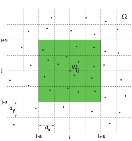
distance between evaluation point and data points unlike the previous methods. This is achieved by mapping sample data to grid point and calculating their distribution using simple raster scan method. When the sample data is mapped into grid point, one more points can be mapped into the same grid point. In this case we take their average value for each x, y, z component as representa-tive and index it. For eachω ∈W, we can find the numbers of grids from ωij
to nonzero grid point along right, left, up and down direction, denoting it by
qr
ω, qlω, quω, qωd, respectively. And then we setqω= 14(q
r
ω+qlω+qωu+qωd). By taking
q= maxω∈W(qω), we can set
h=q·max(dx, dy) (7)
Ω
i i+s
i-s
w
j-s j j+s
dx dy
ij
Fig. 1.DomainΩand local extracted sample data domain
Next, sample data is chosen locally within window of size 2s×2s, where
s= [√3
2 ·q], (8)
centered at each evaluation point ω and [ ] denotes the Gauss’s symbol. This comes from the property of the weight function related to Gaussian function and the relation between h and q. Actually the standard deviation σ in Gaussian function is related to h, like 2σ2
=h2
to the accuracy of the approximated function, we can get the above equation (8). Under these initial conditions, we extract the local subdata set consisted with the above representative data. Since the wanted degree of approximated function is 3, we must increase the magnitude of sby one until the number of data in subdata set is greater than 10. Using this the final local subdata, we calculate the coefficient vector.
2.2 Adaptive h local MLS for data with holes
If the sample data have big holes, the above fixed halgorithm is unsuitable to reconstruct the original image as shown in Fig. 4 (b),(c). Larger the size of holes is, bigger his taken. Then the dense part, like nose, eyes and lips, are getting to lose their characteristic property. Therefore, we do not use global q but use localqω for eachω∈W. Then the adaptivehω
hω=qω·max(dx, dy) (9)
and the initial adaptivesω
sω= [
3 √
2·qω]. (10)
Under the adaptive initial conditions, we follow the same process as fixed algorithm. Refer the experimental results in section 3.4.
3
Experimental results and conclusions
3.1 Reconstruction accuracy
In this section we demonstrate the accuracy of our proposed algorithm by the use of 5 test function as follows:
g1(x, y) = 0.75 exp[−((9x−2)
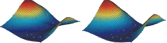
wherex, yare in the domain [0,1]. We perform experiments with some sample data generated randomly in [0,1]. Here M100 and M500 means 100 and 500 sample data with 49 and 625 uniform data respectively, while others are ran-domly sampled. On the other hand R500 is 500 totally random data. Fig. 2 is the feature ofg3and its approximated image. The points on the surface are the sample data for M100 case. For each test functiongi, we can find the accuracy
error which is divided the RMS error by the difference if maximum and minimum values ofgi between the function values on a dense grid. That is,
RMS = s
Pnx i=0
Pny
j=0(gi(xi, yi)−f(xi, yj))2
(nx+ 1)(ny+ 1)
,
wherexi =i/nx, y =j/nyandnx=ny = 50. Under the sameh, we compare the
RMS values for each case. Table 1 shows that the fact that MLS approximation theory does not need to have the whole data(WD) but is enough only local data(LD).
Fig. 2.Feature ofg3(left) and its approximated image for M100(right)
Table 1.Comparison of RMS error between WD and LD for M100, M500 and R500
M100 g1 g2 g3 g4 g5
WD .01076 .00694 .00070 .00199 .00020 LD .01085 .00699 .00070 .00201 .00020
M500 g1 g2 g3 g4 g5
WD .00079 .00047 .00004 .00013 .00001 LD .00089 .00045 .00005 .00018 .00001
R500 g1 g2 g3 g4 g5
WD .00080 .00143 .00009 .00020 .00002 LD .00089 .00152 .00009 .00022 .00004
3.2 Time complexity
Table 2.Time complexity between whole data and local data
Time (sec) M100 M500
WD 10.64 46.22
LD 7.32 9.42
3.3 Filling holes with adaptive h local MLS
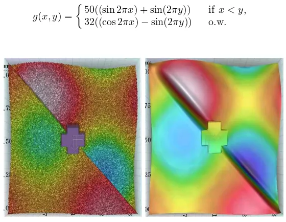
Firstly we have experimented forgwith additive random noise data of magnitude 20 and some data in original data set is removed to have one hole of the cross shape.
g(x, y) = ½
50((sin 2πx) + sin(2πy)) if x < y,
32((cos 2πx)−sin(2πy)) o.w.
Fig. 3. g function with cross hole by generating noise(left) and its filling hole im-age(right)
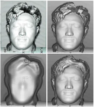
Although the given surface is smooth, if it has missing data with the big sized hole, then fixedhlocal MLS algorithm is unsuitable. Next, we experiment with real face range data having many noisy data and very big holes. If we take the large fixed hfrom the largest hole, it can work well for filling holes but it cannot preserve the details. but if we use the adaptive hlocal algorithm, then we get the nice result like Fig. 4 (d).
3.4 Conclusions and further studies
By introducinghadaptively in every evaluation points, we get the smooth surface that preserves the detail parts such as nose, eyes and lips and fills holes nicely. However, this algorithm occurs some discontinuity on the boundary of each hole due to abrupt change ofhnear it. So we are researching about multilevel method for getting more smooth results. Some experimental results give us clues that it is very reasonable guess.
Fig. 4. (a) original face range image, (b) approximated image with fixed h= 3, (c) h= 15 (d) approximated image with adaptiveh
4
Acknowledgements
2. This research was supported by the Program for the Training of Graduate Stu-dents in Regional Innovation which was conducted by the Ministry of Commerce Industry and Energy of the Korea Government
References
1. F. Abramovici, The Shepard interpolation as the best average of a set of data, Technical Report, Tel-Aviv University, 1984.
2. G. Backus and F. Gilbert, The resolving power of gross earth data, Geophys.J.R. Astr. Soc.16169-205, 1968.
3. L. Bos and K. Salkauskas, Moving least-squares are Backus-Gilbert optimal, J. Ap-prox. Theory59(3) 267-275. 1989.
4. D. Levin, The approximation power of moving least-squares, Mathematics of com-putation, vol 67,224, 1517-1531, 1998.