Impact of generalized travel costs on sa

(1)

Procedia - Social and Behavioral Sciences 39 ( 2012 ) 195 – 204

The Seventh International Conference on City Logistics

Impact of generalized travel costs on satellite location in the

Two-Echelon Vehicle Routing Problem

Teodor Gabriel Crainic

a,b

, Simona Mancini

c*

, Guido Perboli

a,c

, Roberto Tadei

c

a_{CIRRELT, Université de Montréal, C.P. 6128, succ. Centre-ville Montréal (Québec) Canada H3C 3J7} b_{École des sciences de la gestion, UQÀM, C.P. 8888, succ. Centre-ville, Montréal (Québec) Canada H3C 3P8}

c_{Politecnico di Torino, Corso Duca degli Abruzzi 24, Torino, 10129, Italy}

Abstract

In this paper we address the Two-Echelon Vehicle Routing Problem (2E-VRP), the variant of VRP where freight is delivered from depots to intermediate satellites, and then it is delivered to customers while minimizing the global routing costs of the overall two-echelon network. The goal of this work is to address more realistic situations in urban freight delivery where the travel costs are not only given by distances, but also by other components, like fixed costs for using the arcs, operational costs, and environmental costs. We introduce a generalized travel cost that may combine different components, e.g., operational, environmental, congestion, etc. We then analyze how the different components of the generalized cost affect the satellite location in the 2E-VRP and whether and under which conditions the Two-Echelon approach dominates the Single-Echelon one.

Keywords: Vehicle Routing; City Logistics; generalized travel costs; Two-Echelon distribution

1.Introduction

In the Two-Echelon Vehicle Routing Problems family, the delivery from one or more depots to customers is performed in two phases: first, freight is delivered to intermediate depots, called satellites, where, it is loaded on smaller vehicles, and, in a second phase, it is delivered to customers. This approach is strongly connected to City Logistics and in particular to two-tier City Logistics systems ([1] and [2]),

*_{Corresponding author. Tel.:+39-34-94326879; fax: +39-01-15647099.}

E-mail address: simona.mancini@polito.it

(2)

which build on and expand the City Distribution Center (CDC) idea [3], used in the context of City Logistic by the introduction of Urban Distribution Centers and Urban Consolidation Centers [4],[5]. CDCs form the first level of the system and are located on the outskirts of the city. The second tier of the system is constituted by satellite platforms, where the freight coming from the CDCs and, eventually, other external points may be transferred to and consolidated into vehicles adapted for utilization inside the city. In more advanced systems, satellites do not perform any vehicle-waiting or warehousing activities, vehicle synchronization and transdock transhipment being in use. Urban vehicles move freight to satellites, possibly by using routes specially selected to facilitate access to satellites and reduce the impact on traffic and environment. They may visit more than one satellite during a trip, and, at the end of their route, they are supposed to come back to the CDC. City freighters are environmental friendly vehicles of relatively small capacity, which are allowed to travel along any street in the city to perform all required distribution activities at the second level of the system. The importance of using this kind of vehicles is twofold. In fact, the pollution due to their use is very limited, and this could contribute to have a better air quality in the city centers, while the limited dimensions of the vehicles allow reaching each point of the city, including in historical cities characterized by downtown narrow streets. This approach has already been used in several European cities with good profit. There are still many open issues related to this problem, including most CDC and satellite location issues (see [6], where a pioneering contribution is given, and [7] where the Two-Echelon location routing problem is addressed).

In previous works, the attention was mainly focused on the minimization of the total traveled distance. Even if the distance plays a crucial role in cost computation, it is not the only parameter which influences it. Other important parameters are the typology of the arc (highway, city center street, etc.), and the type of vehicle covering it. Furthermore, if we also consider environmental issues, the perception of costs can sensibly change. In fact, the use of smaller environment friendly vehicles can results in higher costs, both because the high technology necessary to produce these vehicles has a non negligible cost, and because, using smaller vehicles, we need to increment the size of the fleet to perform all the deliveries.

Nevertheless, in a City Logistics context we may prefer to use smaller vehicles, looking at the increment of real cost as the price to pay for a better air quality. In this case, we would assign smaller costs to these types of vehicles, in order to promote their use. The goal of this work is to address more realistic situations in city freight delivery where the travel costs are not only given by distances, but also by other components, like fixed costs for using the arcs, operational costs, and environmental costs.

More in detail, we want to analyze how these more comprehensive travel costs affect the satellite location in the 2E-VRP and whether and under which conditions the Two-Echelon approach dominates the Single-Echelon one. In particular, it is of great interest to analyze the behavior of our approach when we want to minimize the emission of CO2. In this case, the arc costs are time dependent, as they depend

on the traffic congestion, which varies over time, other than geographically.

We first define a generalized cost function as a linear combination of different parameters: the length of the arc, the toll which may be requested for entering the arc (generally a fixed toll, not dependent on the arc length), and the travelling time, which is time dependent. We present different sets of experiments in which we analyze different scenarios generated by varying the cost definition rule and we provide a detailed analysis on the variation of satellite usage. Furthermore, our results will be compared with those obtained with a Single-Echelon distribution system and the impacts of the typology of costs on the location aspects are also investigated.

2. Problem statement

(3)

x freight arrives to the depot, where it is consolidated into the 1st-level vehicles;

x each 1st-level vehicle travels to a subset of satellites, and then returns to the depot;

x at each satellite, freight is transferred from 1st-level vehicles to 2nd-level vehicles;

x each 2nd-level vehicle starts from a satellite, performs a route to serve the designated customers, and then returns to the same satellite for its next cycle.

The goal is to serve customers by minimizing the total transportation cost, and satisfying the capacity constraints of vehicles and satellites.

We consider a single depot and a fixed number of capacitated satellites. Vehicles capacity is homogeneous for vehicles operating at the same level, while it varies among levels.

Customer demands are fixed and known in advance and must be satisfied (no rejection of customers is allowed). No time windows are defined for deliveries and satellites are assumed to be available at each time of the day. The demand of each customer is supposed to be smaller than the vehicle capacity and cannot be split at any level. At the 1st level, a satellite can be served by different vehicles, which means that the aggregate satellite demand can be split.

A general time-dependent formulation with fleet synchronization and customer time windows was introduced in [8] within the context of Two-Echelon City Logistics systems. The authors indicated promising algorithmic directions, but no implementation was reported.

A formal definition of Multi-Echelon VRP problems, a flow model and valid inequalities have been presented in [9]. Instances up to 32 customers were solved to the optimum and instances up to 50 customers solved to near optimality. The authors introduced two math-heuristics able to address instances up to 50 customers within reasonable computational time. Some of these instances have been solved by the Branch and Cut proposed in [10]. Concerning heuristic methods, the fast clustering heuristic of [11] provides the means to address larger instances (up to 250 customers). In this method, the first and the second level are separately considered.

Customers are first assigned to the nearest available satellite, then the second level problem is split into several single-depot VRPs, one for each satellite, where the satellite is considered as depot and only the customers assigned to that satellite are considered. The second level solution is used as input for the first level problem, which is treated as a split delivery VRP, where the satellites are considered as the customers of the depot. The demand of each satellite is computed as the sum of the demands of the customers assigned to it. A multi-start heuristic presented in [12] allows finding good solutions in short computational times.

In [1] a deep analysis of the layout impact on distribution costs is given. The analysis focuses on the impact of several parameters, directly correlated to the instance layout, like the number of customers, number of satellites, customers distributions and satellite locations. The comparison with the Single Echelon distribution approach shows that the Two-Echelon approach is strongly preferable, because it allows to significantly reduce the total transportation cost, computed as the pure distance cost.

Nevertheless, when the travel cost is not only given by the distance and other cost components are considered, the dominance of the Two-Echelon approach vs. the Single-Echelon one is no more so evident and this issue should be carefully analyzed.

3. A generalized cost function

(4)

ܿ_௜௝௩௛ ൌ ߙܭ_௜௝ᇱ ൅ ߚܭ_௜௝ᇱᇱ௩൅ ߛܭ_௜௝ᇱᇱᇱ௩ݐ_௜௝௛

The first cost ܭ௜௝ᇱ is a fixed cost related to the usage of the arc (i,j), e.g. a road toll that must be paid

for using that arc. Typically, if we consider a urban area, the first level arcs could be subject to road toll, while the second level ones are not. But there are some real cases, e.g. Singapore and London, where a high toll must be paid to access downtown in order to limit the traffic congestion in the central zone.

More in detail, tolls related to arcs connecting the CDC to a satellite, generally belonging to a highway, are much higher than tolls related to arcs connecting two depots, which may belong to a motorway or a ring road around the city. This situation is typical of some European cities (and Italian ones in particular). Furthermore, tolls may also sensibly vary with the size of the vehicle, but, since in our problem each arc can be covered by one kind of vehicles only, we do not consider this case. The second cost represents the operational cost, given by the arc length dij multiplied by a parameter ܭ௜௝ᇱᇱ௩ whose

value depends on the vehicle type v and on the geographical position of the arc itself. In fact, larger vehicles generally have a larger cost per km (fuel, depreciation charge, etc.) and highways and motorways, in which vehicles can maintain a constant cruise speed, have a smaller cost per km, under the same traffic conditions, with respect to city streets in which the vehicle is subject to continuous accelerations and decelerations due to traffic lights and traffic congestion.

The third term of the generalized travel cost, which can be addressed as an environmental cost, is related to the pollution emission for using arc (i,j) in a particular day-hour h and can be represented by the average travel time ݐ_௜௝௛ to cover the arc during day-hour h multiplied by a coefficient ܭ_௜௝ᇱᇱᇱ௩proportional to the quantity of the pollution emitted by the vehicle type v in a time unit when using that arc. This coefficient is influenced both by the typology of the arc (highway, main street, small street, etc.) and by the typology of the vehicle.

The term ݐ_௜௝௛ allows us to also consider the traffic congestion, which varies over time and plays an important role in the arc cost computation. In fact, congestion is strictly time-dependent and is structured in different layers moving in concentric circles from the city center outwards and vice versa (for a deeper analysis of these aspects we refer to [13]). Values of the CO2 emission for different types of vehicles,

different types of roads, and different average speeds can be found in [14]. Data on the relation between the arc traveling time ݐ_௜௝௛and the level of traffic congestion can be found in [15]. We consider this third term of the generalized cost function as a separate entity with respect to the second term. In fact, even if in most cases the travel time associated to an arc is linear dependent on its length, there are cases in which this is not true. Since we identify the arc between two entities of the problem with the shortest path connecting them, this path can be composed of different types of roads; in this case, the travel times do not linearly depend on distances. Furthermore, the same arc can have different travel times in different hours of the day, even if we do not consider the traffic congestion level. In fact, traffic lights, which slow down the average speed of the vehicle and consequently the travel time, generally are turned off during night hours. For all these reasons we decided to keep separate, in the generalized cost function, the term dependent on the distances and the term dependent on the travel time.

4. Plan of experiments

In this section we describe our plan of experiments. In order to analyze different realistic cases, we developed various scenarios, which can be grouped as follows:

(5)

x Analysis of costs with fixed tolls:in this case we consider (D = E = 1, J = 0). We address two different scenarios. In the first one, we consider high tolls for arcs connecting the depot and the satellites and small tolls for arcs between two satellites, while the second level arcs are considered free of charge. In the second case, we assign high tolls to arcs inside the city centers, while all the others are considered

free of charge (Singapore’s model).

x Analysis of different traffic conditions:in this case all the terms of generalized cost function are taken into consideration (D = E = J=1). Three different scenarios have been generated, each one representing a different part of the day, early morning, early afternoon, and late afternoon.

Each scenario is composed of 9 instances, with 50 customers and 5 satellites, characterized by a different combination of customer distribution (random, centroids, quadrants) and satellite location (random, sliced, forbidden). For more details about the instances, we refer to [1]. The number of vehicles for the second level has been incremented by one unit in order to easily get a quite large number of feasible solutions. We used the fast clustering heuristic in [9] to perform our experiments.

For each scenario we analyze the impact of the cost definition on the variation of total cost according to the different customer distributions and satellite locations, and we analyze how the cost definition influences the satellite usage.

Opening fixed costs of the satellites are not considered in this study because they do not influence the parameters we want to analyze. They could be treated as an additive constant in the objective function, as they do not depend on the satellites usage.

More details on the scenario parameters are given in the next section.

5. Analysis of distance based costs

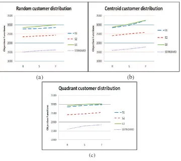
Three different scenarios S1, S2 and S3 have been generated. In S1 we consider costs depending on vehicles. A first level vehicle has a cost per km which is considered 2.5 times greater than a second level one. For that reason we have assumed that= 1 for all the arcs belonging to the second level and ܭ_௜௝ᇱᇱ= 2.5 for the arcs belonging to the first one. If we analyze costs depending on the type of road, as in S2, the relation among the levels is completely reversed; in fact, we consider ܭ௜௝ᇱᇱ= 1 for all the arcs belonging to

the first level, ܭ_௜௝ᇱᇱ= 1.5 for large streets inside the city (suburbs) and ܭ_௜௝ᇱᇱ= 2 for downtown arcs. In S3 we take into account both vehicle and arc typology assigning the following values to the parameter ܭ_௜௝ᇱᇱ: ܭ_௜௝ᇱᇱ= 2.5 for all the arcs belonging to the first level, ܭ_௜௝ᇱᇱ= 1.5 for large streets inside the city (suburbs), and ܭ_௜௝ᇱᇱ= 2 for downtown arcs. All this data are taken from [14]. In Fig. 1 we report the optima for each scenario and for the standard cost computation case, namely STANDARD, i.e. the cost obtained forcing ܭ_௜௝ᇱᇱ=1 for every arc. In Fig. 2 we report a graphical view of the gap among the objective functions related to different satellite locations, letting fixed the customer distribution. On the X axes, the letters R, S and F correspond respectively to random, sliced and forbidden satellites location.

(6)

small discrepancy between real and modeled costs does not have negative effects on the best solution search.

Fig. 1. Distance based cost scenario optima

(a)

(b)

(c)

(7)

Fig. 3. Satellite usage for scenarios S1, S2 and S3

6.Analysis of costs with fixed tolls

In this section we analyze cases in which a fixed toll must be paid for using some arcs. This is a very common policy in the many cities (highway, city center entrance tolls, etc.). These toll types are generally paid to enter a particular road or zone, and they do not depend on distance. Cases in which the toll is dependent on the distances can be treated as the scenarios presented in the previous section.

We analyze two possible scenarios: one representing a typical Italian and European city, the other one representing a city in which high toll must be paid for entering downtown (like Singapore). In scenario S4 we consider high tolls, ܭ_௜௝ᇱ=20, for arcs connecting the depot to the satellites and smaller tolls, ܭ_௜௝ᇱ=5 for arcs between two satellites, while the second level arcs are considered free of charge. In the second one, S5, downtown arcs have a fixed toll (very high)ܭ_௜௝ᇱ=10 and other arcs are free of charge. Since, from the previous section, we know that the value of ܭ_௜௝ᇱᇱ௩is not so relevant, we consider ܭ_௜௝ᇱᇱ௩=1 for all arcs.

(8)

In Fig. 4, we report the satellite usage for S4 and S5. First, we can notice that, in S4, the distribution of goods is equal to the one obtained in the STANDARD case. This can be easily justified by analyzing the impact of tolls on the distribution. Direct arcs from depot to satellites have a greater cost with respect to those between satellites. This implies that at the first level, routes serving more satellites are preferred to routes serving one satellite only.

This means that, the first level solution can appear completely different with respect to the standard case, but it does not have any effect on the satellite usage, and consequently on the second level routing. Instead, in S5, the distribution is quite uniform among satellites. This behavior coincides on what we would have expected. In fact, because of the high cost of central arcs, the minimization of total cost would avoid to use them, as much as possible. For doing that, each customer is assigned to a satellite located in the same part of the city from which it can be reached without crossing the center. This kind of solution can be used with profit in many real applications, where the best solution in term of distance, generally does not correspond to the most advantageous one.

7. Analysis of different traffic conditions

In this section, we present three different temporal scenarios, each one of them representing a different part of the day, with the related traffic conditions. The first one, S6, represents a typical early morning situation, in which incoming arcs are heavily congested, outgoing arcs are subjected to normal traffic conditions while downtown arcs are lightly congested. The second one, S7, represents a late afternoon situation, in which outgoing arcs are heavily congested, incoming arcs are subjected to normal traffic conditions, while downtown arcs are heavily congested. Finally, the last scenario S8, represents an early afternoon situation, where downtown arcs are congested, while the other arcs have a normal traffic condition. All the scenarios represent situations related to a standard working day, while during weekends, holidays, or summer periods, traffic conditions may be different. For heavily congested arcs we consider a travel time 3 times greater than in normal conditions. For congested arcs the travel time is doubled and for light congested arcs it is 1.5 times higher.

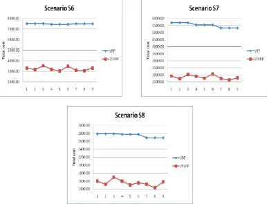
In Fig. 5, we report the results obtained on scenarios S6, S7 and S8 while the two last columns (gain) report, respectively the percentage cost reduction obtainable performing the delivery in the late afternoon (S7) and in the early afternoon (S8) with respect to doing it in the early morning (S6). As we can easily observe, there is a very strong cost reduction in both cases (between 40 and 46% for S7 and between 50 and 53% for S8), but the highest reduction is obtained by performing the delivery operations in the early afternoon. Nevertheless, this strategy cannot be actuated in all the situations because in several real applications (like bread and fresh pastries delivery, newspaper delivery etc.) goods shall be delivered in the early morning. For a global reduction of costs, delivery operations not subjected to this particular constraint could be performed in the afternoon, reducing the traffic congestion in the early morning, in which the activities requested must be performed with lower costs.

(9)

using a fleet of vehicles equal to the vehicles used in the second level of the 2E-VRP. If we compare the 2E-VRP with the standard VRP we can notice that our approach is always strongly preferable because it allows, for all the scenarios, an average cost reduction of 55% with respect to the standard VRP method. The best gain is obtained on S7 and S6 where the depot-to-city connection costs are higher. In fact, in the standard VRP approach, vehicles are obliged to come back to the depot at the end of each route, which implies a larger use of incoming (S6) and outgoing (S7) arcs, which yields high costs. Even in S8, where higher costs are related to central arcs, the gain of our approach is still large (around 43%).

Fig. 5. Comparison with the VRP approach for scenarios S6, S7 and S8

(10)

The results show that the Two-Echelon approach is better than the Single-Echelon one in all the cases we analyzed, keeping in mind that we are not considering opening fixed costs for the satellites, which would increase the 2E-VRP global cost. Nevertheless, the gain obtained following the Two-Echelon approach is so large that, even adding these opening costs, this distribution strategy should be preferable.

8.Conclusion

In this paper, we analyzed how different travel costs may affect the satellite location in the 2E-VRP and if this approach is preferable to the Single-Echelon one. A detailed analysis of computational results shows that the satellite usage is not affected by the increasing of incoming and/or outgoing arc costs, while, when the downtown arc costs increase, the satellite usage strongly change, assuming a configuration with a uniform demand distribution among satellites. The 2E-VRP approach performs better than the classical VRP. A further reduction of cost can be obtained by performing the delivery operations in the afternoon, reducing the traffic congestion in the early morning, when the deliveries which are strictly requested to be performed can be made at lower costs.

References

[1] Crainic TG, Mancini S, Perboli G, Tadei R.Two-Echelon Vehicle Routing Problem: A satellite location analysis. Procedia Social and Behavioral Sciences 2009;2: 5944-5955.

[2] Benjelloun A, Crainic TG. Trends, challenges and perspectives in City Logistics. In: Transportation and land use interaction,

Proceedings TRANSLU’08, Editura Politecnica Press, Bucharest, Romania; 2008, p. 269-28.

[3] Duin JHR van. Evaluation and evolution of the city distribution concept. In: Urban transport and the environment for the 21st

Century III, WIT press, Southampton;1997, p.327-337.

[4] Allen J, Thorne G, Browne M. BESTUFS Good practice guide on urban freight transport. BESTUFS consortium; www.bestufs.net; 2000.

[5] Browne M, Sweet M, Woodburn A, Allen J. Urban freight consolidation centres. Transport Studies Group, University of Westminster, London; 2005.

[6] Crainic TG, Ricciardi N, Storchi, G. Advanced freight transportation systems for congested urban areas. Transportation Research Part C, Emerging Technologies 2004; 12: 119-137.

[7] Boccia M, Crainic TG, Sforza A, Sterle C. A metaheuristic for the two-echelon location routing problem. Lecture Notes in Computer Sciences 2010; 6049: 288-301.

[8] Crainic TG, Ricciardi N, Storchi G. Models for evaluating and planning City Logistics systems. Transportation Science 2009; 43: 432-454.

[9] Perboli G, Tadei R, Vigo D. The two-echelon capacitated vehicle routing problem: models and math-based heuristics

Transportation Science 2011;doi: 10.1287/trsc.1110.0368, forthcoming.

[10] Masoero F, Perboli G, Tadei R. New Families of valid inequalities for the two-echelon vehicle routing problem Electronic Notes in Discrete Mathematics 2010;36: 639-646.

[11] Crainic TG, Mancini S, Perboli G, Tadei R. Clustering-based heuristics for the two-echelon capacitated vehicle routing problem. Publication CIRRELT-2008-46, CIRRELT, Montréal, Canada; 2008.

[12] Crainic TG, Mancini S, Perboli G, Tadei R. Multi-start heuristics for the two-echelon vehicle routing problem.Lecture Notes in Computer Science 2011; 6622: 179-190.

[13] Stathopoulos A, Karlaftis, M. Temporal and spatial variation of real-time traffic data in urban areas. Transportation Research Record, Journal of the Transportation Research Board 2007; 1768/2001:135-140.

[14] Cappiello A. Modeling traffic flow emissions. Master’s thesis, Environmental Engineering, Politecnico di Milano, Italy; 1998. [15] Alta Scuola Politecnica . Digital Logistics: Transforming regional-scaled freight logistics with digital integration. AS project’s