MATA KULIAH
PENGANTAR TEKNIK INFORMATIKA
Universitas Mercu Buana Yogyakarta
Kuliah E-Learning
Tugas Elearning TTM 05
(Pertemuan Kelima)
Tugas :
Pelajarilah materi Computational Science, kemudian saudara deskripsikan
dengan singkat (tidak lebih dari satu halaman A4) mengenai Computational
Science yang di paparkan dalam materi sessi ini.
Tugas dikirim via email :
[email protected], dan telah masuk ke inbox
tidak lebih dari 5 hari dari sessi ini. Dengan Subject
<NIM>_<NAMA>_<MATAKULIAH>
III
Computational
Science
Computational Science unites computational simulation, scientific experimentation, ge-ometry, mathematical models, visualization, and high performance computing to address some of the “grand challenges” of computing in the sciences and engineering. Advanced graphics and parallel architectures enable scientists to analyze physical phenomena and processes, providing a virtual microscope for inquiry at an unprecedented level of detail. These chapters provide detailed illustrations of the computational paradigm as it is used in specific scientific and engineering fields, such as ocean modeling, chemistry, astrophysics, structural mechanics, and biology.
26 Geometry-Grid Generation Bharat K. Soni and Nigel P. Weatherill
Introduction • Underlying Principles • Best Practices • Grid Systems • Research Issues and Summary
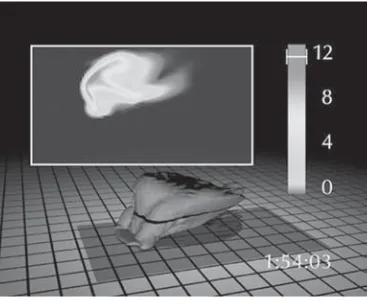
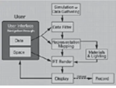
27 Scientific Visualization William R. Sherman, Alan B. Craig,
M. Pauline Baker, and Colleen Bushell
Introduction • Historic Overview • Underlying Principles • The Practice of Scientific
Visualization • Research Issues and Summary
28 Computational Structural Mechanics Ahmed K. Noor
Introduction • Classification of Structural Mechanics Problems • Formulation of
Structural Mechanics Problems • Steps Involved in the Application of Computational
Structural Mechanics to Practical Engineering Problems • Overview of Static, Stability,
and Dynamic Analysis • Brief History of the Development of Computational Structural
Mechanics Software • Characteristics of Future Engineering Systems and Their
Implications on Computational Structural Mechanics • Primary Pacing Items and
Research Issues
29 Computational Electromagnetics J. S. Shang
Introduction • Governing Equations • Characteristic-Based Formulation • Maxwell Equations in a Curvilinear Frame • Eigenvalues and Eigenvectors • Flux-Vector Splitting • Finite-Difference Approximation • Finite-Volume
Approximation • Summary and Research Issues
30 Computational Fluid Dynamics David A. Caughey
Introduction • Underlying Principles • Best Practices • Research Issues and Summary
31 Computational Ocean Modeling Lakshmi Kantha and Steve Piacsek
Introduction • Underlying Principles • Best Practices • Nowcast/Forecast in the Gulf
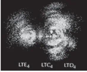
32 Computational Chemistry Frederick J. Heldrich, Clyde R. Metz, Henry Donato, Kristin D. Krantzman, Sandra Harper,
Jason S. Overby, and Gamil A. Guirgis
Introduction • Computational Chemistry in Education • Computational Aspects of
Chemical Kinetics • Molecular Dynamics Simulations • Modeling Organic
Compounds • Computational Organometallic and Inorganic Chemistry • Use ofAb Initio
Methods in Spectroscopic Analysis • Research Issues and Summary
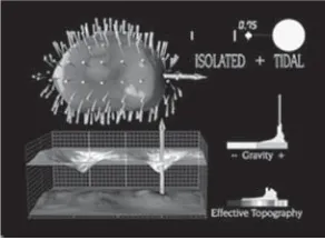
33 Computational Astrophysics Jon Hakkila, Derek Buzasi, and
Robert J. Thacker
Introduction • Astronomical Databases • Data Analysis • Theoretical Modeling • Research Issues and Summary
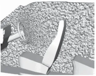
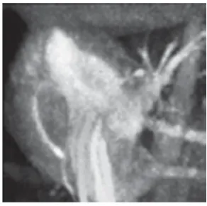
34 Computational Biology David T. Kingsbury
Introduction • Databases • Imaging, Microscopy, and Tomography • Determination of
26
Geometry-Grid
Generation
Bharat K. Soni
Mississippi State University
Nigel P. Weatherill
University of Wales Swansea
26.1 Introduction
Structured Grids • Unstructured Grids •Generation Process
26.2 Underlying Principles
Terminology and Grid Characteristics• Geometry Preparation •Structured Grid Generation •Unstructured Grid Generation
26.3 Best Practices
Structured Grid Generation • The Delaunay Algorithm •Hybrid Grid Generation
26.4 Grid Systems
26.5 Research Issues and Summary
26.1 Introduction
With the advent and rapid development of supercomputers and high-performance workstations, compu-tational field simulation (CFS) is rapidly emerging as an essential analysis tool for science and engineering problems. In particular, CFS has been extensively utilized in analyzing fluid mechanics, heat and mass transfer, biomedics, geophysics, electromagnetics, semiconductor devices, atmospheric and ocean science, hydrodynamics, solid mechanics, civil engineering related transport phenomena, and other physical field problems in many science and engineering firms and laboratories.
The basic equations governing the general physical field can be represented as a set of nonlinear partial differential equations pursuant to a particular set of boundary conditions. For computational simulation, the field is decomposed into a collection of elemental areas (2-D)/volumes (3-D). The governing equations associated with the field under consideration are then approximated by a set of algebraic equations on these elemental volumes and are numerically solved to get discrete values which approximate the solution of the pertinent governing equations over the field. This discretization of the field (domain, region) into finite-elemental areas/volumes is referred to as grid generation, and the collection of discretized elemental areas/volumes is called the grid.
1983]. The differential forms of the governing equations are utilized in this case. However, the integral forms of the governing equations are used in the cases of finite-element and finite-volume strategies. Here the solution process involves representation of the solution variables over the cell in terms of selected functions, and then these functions are integrated over the volume (in case of finite-element) or the associated fluxes through cell sides (edges) are balanced (in case of finite volume).
The finite-element approach itself comes in two basic forms — thevariational, where the PDEs are replaced by a more fundamental integral variational principle (from which they arise through the calculus of variations), or theweighted residual(Galerkin) approach in which the PDEs are multiplied by certain functions and then integrated over the cell.
In the finite-volume approach the fluxes through the cell sides (which separate discontinuous solution values) are best calculated with a procedure which represents the dissolution of such a discontinuity during the time step (Riemann solver).
The finite-difference approach, using the discrete points, is associated by many with rectangular Carte-sian grids since such a regular lattice structure provides easy identification of neighboring points to be used in the representation of derivatives, whereas the finite-element approach has always been, by the nature of its construction on discrete cells, considered well-suited for irregular regions since a network of cells can be made to fill any arbitrarily shaped region and each cell is an entity unto itself, the representation being on a cell, not across cells. In view of the discretization strategy employed, the grids can be classified as structured, unstructured, or hybrid.
26.1.1 Structured Grids
Letr=(x,y,z) andΩ=(,,) denote the coordinates in the physical and computational space. The structured grid is presented by a network of lines of constant,, andsuch that a one-to-one mapping can be established between physical and computational space. The computational space is made up of uniformly distributed points within a square in two dimensions or a cube in three dimensions as demonstrated in Figure 26.1. The structured grid involving identity transformation between physical and computational space (that is,x=,y=,z=) is called a Cartesian grid. However, the body-fitted grid generated by utilizing discrete/analytic arbitrary transformations between physical and computational space is classified as a curvilinear grid. A grid around a cylinder demonstrating the Cartesian grid and curvilinear two-dimensional grid demonstrating O, C, and H type strategies and their respective correspondence with the computational domain are displayed inFigure 26.2athrough Figure 26.2d.
The curvilinear grid points conform to the solid surfaces/boundaries and hence provide the most economical and accurate way for specifying boundary conditions. For example, in the O-type grid the boundary of the cylinder is specified at=1 boundary, and=1 and=maxboundaries represent the same physical boundary (commonly referred to as a cut line). In the C-type grid the cylinder boundary is mapped into only a part of theboundary, as shown in the Figure 26.2c. Here, the boundary segment in the front of the airfoil in the computational domain and at the tail of the airfoil represent the cut line
(b)
(c) (d) (a)
FIGURE 26.2 (a) Cartesian grid, (b) O-type grid, (c) C-type grid, and (d) H-type grid.
(a) (b)
FIGURE 26.3 (a) Multiblock grid showing matching, nonmatching, and overlapping strategies and (b) overlaid chimera grid.
boundary. However, in the H-type grid an airfoil is mapped into the middle of the computational domain as shown in Figure 26.2d.
For complicated geometrical configurations, the physical region is divided into subregions, within each of which a structured grid is generated. These subgrids are commonly referred to as composite grids, and the generation process is referred to as domain decomposition [Thompson 1987b]. The resulting subgrids may be patched together at common interfaces, may be overlapped, or may be overlaid. Self-explanatory pictorial views of domain decomposition strategies allowing patched blocks, overlapping blocks, and overlaid blocks are presented in Figure 26.3a and Figure 26.3b. Overlaid grids are also called chimera grids after the composite monster of Greek mythology.
FIGURE 26.4 Unstructured grid.
variables may not satisfy the conservation requirement associated with the overall simulation process, resulting in spurious oscillations in the vicinity of the interface.
In general, the composite grids are presented as
ri j kl(i=1,. . .,IMAX (l), j =1,. . .,JMAX (l), k=1,. . .,KMAX (l), l =1,. . .,NBLKS) wherei,j, andkidentify three curvilinear coordinates,IMAX(l),JMAX(l),KMAX(l) denote the grid dimensions in each direction of blockl.NBLKS represents the total number of blocks and vectorrcontains the physical variables inx,y, andzdirection. In structured grid generation the connections between points are automatically defined from the given (i,j,k) ordering. Such ordering (structure) does not exist in unstructured grids. Unstructured grids are composed of triangles in two dimensions and tetrahedrons in three dimensions. Each elemental volume is called a cell. The grid information is presented by a set of coordinates (nodes) and the connectivity between the nodes. The connectivity table specifies connections between nodes and cells. A pictorial view of a simple unstructured grid is presented inFigure 26.4.
26.1.2 Unstructured Grids
26.1.2.1 Hybrid Grid
A grid formed by a combination of structured–unstructured grids and/or allowing polygonal cells with different numbers of sides is called a hybrid or generalized grid. An usual practice is to generate structured grids near solid components up to desired distance and fill in remaining regions with unstructured (triangular/tetrahedron) grids. A typical hybrid grid is displayed inFigure 26.5.
26.1.3 Generation Process
Regardless of which grid strategy is being considered, creation of a computational grid requires the fol-lowing:
1. Computational mapping:Establishing an appropriate mapping from physical to computational space allowing proper multiblock strategies in case of structured and hybrid grids or establishing an ordering of nodes in case of unstructured grids and hybrid grids.
2. Geometry generation:Defining an accurate numerical description of all solid components (surfaces) in conjunction with associated computational mapping criteria and a desired distribution of points. 3. Computational modeling:Generating anappropriategrid around these surfaces according to some criteria, usually with a specified multiblock strategy, point distribution, smoothness, and orthogo-nality in case of structured grids and desired background mesh representative of point distribution in case of unstructured grids.
FIGURE 26.5 Hybrid grid.
the geometry with the proper distribution of points usually consumes 85 to 90 percent of the total time spent on the grid generation process. The geometry specification associated with grid generation involves the following:
1. Determine the desired distribution of grid points. This depends upon the expected flow character-istics.
2. Evaluate boundary segments and surface patches to be defined in order to resolve an accurate mathematical description of the geometry in question.
3. Select the geometry tools to be utilized to define these boundary segments/surface patches. 4. Follow an appropriate logical path to blend the aforementioned tasks obtaining the desired
dis-cretized mathematical description of the geometry with properly distributed points.
The accuracy of the numerical algorithm depends not only on the formal order of approximations but also on the distribution of grid points in the computational domain. The grid employed can have a profound influence on the quality and convergence rate of the solution. Grid adaption offers the use of excessively fine, computationally expensive, grids by directing the grid points to congregate so that a functional relationship on these points can represent the physical solution with sufficient accuracy.
Underlying principles and methodologies for grid generation and adaption follow.
26.2 Underlying Principles
26.2.1 Terminology and Grid Characteristics
The differencing and solution techniques involving Cartesian (regular) grids are well developed and well understood. The use of structured curvilinear grids (nonorthogonal in most cases) in the numerical solution of PDEs is not, in principle, any more difficult than using Cartesian grids. This is accomplished by transforming the pertinent PDEs from the physical space to computational space. The following notations will be utilized in the development of structured grids and these transformations; detailed mathematical analysis can be found in Thompson et al. [1985]:
r=(x,y,z)≡(x1,x2,x3) =physical space Ω=(,,)≡(1,2,3)
=computational space ai=ri, i=1, 2, 3 =covariant base vectors
ai= ∇i
, i=1, 2, 3 =contravariant base vectors
gi j =ai·aj (i=1, 2, 3), (j =1, 2, 3)=covariant metric tensor components gi j =ai·aj (i=1, 2, 3), (j =1, 2, 3)=contravariant metric tensor components
√
Also it can be shown that for any tensoru
Although Equation 26.1 and Equation 26.2 are equivalent expressions, the numerical representations of these two forms may not be equivalent. The form given by Equation 26.1 is called conservative form and that of Equation 26.2 is called the nonconservative form. Equation 26.1 or Equation 26.2 is utilized for transforming derivatives from physical to computational space. With moving grids the time derivatives also must be transformed using the following equation:
where ˙rindicates the associated grid speed.
The discretization process associated with the finite-volume scheme employed in unstructured or hybrid grids is also very straightforward. Here, the integral equations are utilized. The edge-based data structure is used for connectivity information and can be easily utilized to compute areas of cells and associated fluxes. The area, for example, of a region bounded by a two-dimensional boundary∂is
A=
wherexandyare interpreted as edge quantities. Also, the governing equations are discretized in similar fashion. For example, consider an integral form of the Navier-Stokes equation without body force as follows:
wherenis the outward normal to the control volume with componentsnxandnyin thexandydirections. The domain of interest is discretized into a set of nonoverlapping polygons (unstructured or hybrid grid), and the cell-averaged variables are stored at the cell center. For each cell the semidiscretized form of the governing Equation 26.6 can be written as
Vi where j varies over the cell faces, andFi j andFi jv are the convective and viscous part of the numerical flux at jth edge of celli. Detailed analysis and description of this discretization process can be found in Weatherill [1990] and Koomullil et al. [1996b].
decrease as the point distribution changes. Looking at the truncation error analysis involving nonuniform structured curvilinear grids, the following grid requirements can be outlined: (1) The structured grid system must be either a right-handed system [√g >0 for all (i,j,k)] or a left-handed system [√g <0 for all (i,j,k)]. (2) Application of the distribution function with bounds on higher order derivatives does not change the formal order of approximation. The following functions involving exponential and hyperbolic tangent or hyperbolic sine stretching functions are widely utilized as distribution functions for distributing Npoints:
x()= e
␣(s−1)−1
e␣−1 or x()=1−
tanh(␣(1−s))
tanh(␣) (26.8)
where
s=(−1)/(N−1) 1≤≤N.
(3) Numerical derivative evaluation of the distribution function is preferred, i.e., instead of analytical definition ofx, wherex=[(xi+1−xi−1)/2]. (4) The truncation error is inversely proportional to the sine of the angle between grid lines. This in turn indicates that the mildly skewed grid does not increase truncation error significantly. In fact, as a rule of thumb, nonorthogonality resulting in an angle between grid lines not less than 45◦does not increase truncation errors significantly.
26.2.2 Geometry Preparation
The geometry preparation is the most critical and labor intensive part of the overall grid generation process. Most of the geometrical configurations of interest to practical engineering problems are designed in the computer-aided design/computer-aided manufacturing (CAD/CAM) system. There are numerous geometry output formats which require the designer to spend a great deal of time manipulating geometrical entities in order to achieve a useful sculptured geometrical description with appropriate distribution for grid points. Also, there is a danger of loosing fidelity of the underlying geometry in this process. The desired point distribution on the boundary segment/surface patch is achieved by computing a concentration array of unit length. The concentration array is computed using specified spacing and by selecting an exponential or hyperbolic tangent stretching function. The geometry preparation involves the discrete-sculptured definitions of all outer boundaries/surfaces associated with the domain of interest. In case of unstructured or hybrid grids, the geometry preparation involves the definition of discrete points on the boundaries associated with the domain. The following definitions will be utilized in this development.
Definition 26.1 Given a set of points on a curve with physical Cartesian coordinates (xi,yi,zi),i =
1i,i1+1,. . .,i2. A number sequencer =(r1,r2,. . .,rn), with 0≤rj ≤1, r1=0,rn=1,ri≤rj for all
i < j represents the distribution of points, such that there exists a one-to-one correspondence between the elementrj ofr and the triplet (xj,yj,zj). This number sequencer is called a curve distribution. For example, the normalized chord length withri1=0 and
ri= i
u=i1+1
(xu−xu−1)2+(yu−yu−1)2+(zu−zu−1)2 i2
u=i1+1
(xu−xu−1)2+(yu−yu−1)2+(zu−zu−1)2
(26.9)
wherei=i1+1,. . .,i2 satisfies the definition of a curve distribution.
Definition 26.2 Given a set of points on a surface with physical Cartesian coordinates (xi j,yi j,zi j),i= 1i,i1+1,. . .,i2; j= j1,j1+1,. . .,j2. A mesh (si j,ti j),i=1i,i1+1,. . .,i2; j= j1,j1+1,. . .,j2, is called a surface distribution mesh if (si1j,. . .,si2j) for j= j1,. . .,j2 represents the curve distribution for the curve ((xi j,yi j,zi j), i = i1,i1+1,. . .,i2) for j = j1,j1,. . .,j2) and (ti j1,. . .,ti j2) fori =
i1,. . .,i2 represents the curve distribution for the curve ((xi j,yi j,zi j), j = j1,j1+1,. . .,j2), for
Physical Space Distribution Space Computational Space
FIGURE 26.6 Relationship between physical space, distribution mesh, and computational space.
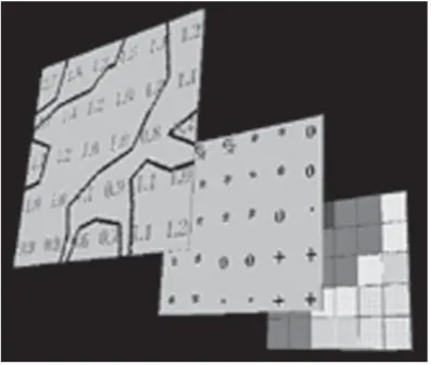
Also, there exists a one-to-one correspondence between the physical domain and the surface distribution mesh and between the surface distribution mesh and the computational domain. These relations are demonstrated inFigure 26.6.
Definition 26.3 Let (Xi j k,Yi j k,Zi j k),i =1, 2,. . .,N; j = 1, 2,. . .,M;k = 1, 2,. . .,L be a single block three-dimensional structured grid. A mesh (si j k,ti j k,qi j k),i =1, 2,. . .,N; j =1, 2,. . .,M;k = 1, 2,. . .,L is called a volume distribution mesh if (si j k,ti j k)i =1, 2,. . .,N; j =1, 2,. . .,Mrepresents the surface distribution mesh for the surface (Xi j k,Yi j k,Zi j k),k =1, 2,. . .,L, (ti j k,qi j k) represents the surface distribution mesh for the surface (Xi j k,Yi j k,Zi j k), for alliand (si j k,qi j k) represents the surface distribution mesh for the surface (Xi j k,Yi j k,Zi j k), for all j.
26.2.3 Structured Grid Generation
26.2.3.1 Algebraic Generation Methods
An algebraic 3-D generation system based on transfinite interpolation (using either Lagrange or Hermite interpolation) is widely utilized for grid generation [Gordon and Thiel 1982, Soni 1992b]. The interpola-tion, in general complete transfinite interpolation from all boundaries, can be restricted to any combination of directions or lesser degrees of interpolation, and the form (Lagrange, Hermite, or incomplete Hermite) can be different in different directions or in different blocks. The blending functions can be linear or, more appropriately, based on the distribution surface/volume mesh. Hermite interpolation, based on cubic blending functions, allows orthogonality at the boundary. Incomplete Hermite uses quadratic functions and, hence, can give orthogonality at any one of two opposing boundaries, whereas Lagrange, with its linear functions, does not give orthogonality.
The transfinite interpolation is accomplished by the appropriate combination of 1-D projectorsFfor the type of interpolation specified. (Each projector is simply the 1-D interpolation in the direction indicated.) For interpolation from all sides of the section, if all three directions are indicated and the section is a volume, this interpolation is from all six sides, and the combination of projectors is the Boolean sum of the three projectors,
F1⊕F2⊕F3≡F1+F2+F3−F1F2−F2F3−F3F1+F1F2F3 (26.10) With interpolation in only the two directions jandk, or if the section is a surface on whichiis constant, the combination is the Boolean sum ofFj andFk
Fj ⊕Fk ≡Fj+Fk−FjFk, (i,j,k) cyclic (26.11) With interpolation in only a single directioni, or if the section is a line on whichivaries, the interpolation is between the two sides on whichiis constant using only the single projectorF
Blocks can be divided into subblocks for the purpose of generation of the algebraic grid. Point dis-tributions on the sides of the subblocks can either be specified or automatically generated by transfinite interpolation from the edge of the side. This allows additional control over the grid in general configura-tions and is particularly useful in cases where point distribuconfigura-tions need to be specified in the interior of a block or to prevent grid overlap in highly curved regions. This also allows points in the interior of the field to be excluded if desired, e.g., to represent holes in the field.
26.2.3.2 Elliptic Generation Method
An elliptic grid generation system [Thompson 1987b] commonly used is
3
i=1 3
l=1
gilril +
3
l=1
gllPlrl =0 (26.12)
where thegil, the elements of the contravariant metric tensor, can be evaluated as
gil= 1
g(gj mgkn−gj ngkm), (i=1, 2, 3), (l =1, 2, 3) (26.13) (i,j,k) cyclic, (l,m,n) cyclic
wheregis the square of the Jacobian.
ThePnare thecontrol functions, which serve to control the spacing and orientation of the grid lines in the field. The first and second coordinate derivatives are normally calculated using second-order central differences. One-sided differences dependent on the sign of the control functionPn(backward forPn<0 and forward forPn>0) are useful to enhance convergence with very strong control functions. The control functions are evaluated either directly from the initial algebraic grid and then smoothed or by interpolation from the boundary point distributions.
The three components of the elliptic grid generation system provide a set of three equations that can be solved simultaneously at each point for the three control functionsPn(n=1, 2, 3), with the derivatives here represented by central differences.
The elliptic generation system is solved by point successive over relaxation (SOR) iteration using a field of locally optimum acceleration parameters. These optimum parameters make the solution robust and capable of convergence with strong control functions.
Control functions can also be evaluated on the boundaries using the specified boundary point distri-bution in the generation system, with certain necessary assumptions (orthogonality at the boundary) to eliminate some terms, then they can be interpolated from the boundaries into the field. More general re-gions can, however, be treated by interpolating elements of the control functions separately. Thus, control functions on a line on whichnvaries can be expressed as
Pn =An+ Sn
̺n
(26.14)
whereAnis the logarithmic derivative of the arc length,Snis the arc length spacing, and̺nis the radius of curvature of the surface on whichnis constant.
The boundary locations are located by Newton iteration on the spline to be at the foot of normals to the adjacent field points.
26.2.3.3 Hyperbolic Generation Method
It is also possible to base a grid generation system on hyperbolic PDEs rather than elliptic equations. In this case, the grid is generated by numerically solving a hyperbolic system [Steger and Chaussee 1980], marching in the direction of one curvilinear coordinate between two boundary curves in two dimensions or between two boundary surfaces in three dimensions. The hyperbolic system, however, allows only one boundary to be specified and is therefore of interest only for use in calculation on physically unbounded regions where the precise location of a computational outer boundary is not important. The hyperbolic grid generation system has the advantage of being generally faster than elliptic generation systems, but, as just noted, is applicable only to certain configurations. Hyperbolic generation systems can be used to generate orthogonal grids. In two dimensions, the condition of orthogonality is simplyg12=0.
If either the cell area√gor the cell diagonal length (squared)g11+g22is a specified function of the curvilinear coordinates, i.e.,
√
g =F(,) or g11+g22=F(,) (26.15) then the system consisting ofg12=0 and either of the preceding two equations is hyperbolic. Since the system is hyperbolic, a noniterative marching solution can be constructed proceeding in one coordinate direction away from a specified boundary.
26.2.3.4 Multiblock Systems
Although in principle it is possible to establish a correspondence between any physical region and a single empty logically rectangular block for general 3-D configurations, the resulting grid is likely to be much too skewed and irregular to be usable when the boundary geometry is complicated. A better approach with complicated physical boundaries is to segment the physical region into contiguous subregions, each bounded by six curved sides (four in 2-D) and each of which transforms to a logically rectangular block in the computational region. Each subregion has its own curvilinear coordinate system, irrespective of that in the adjacent subregions (see Figure 26.7). This then allows both the grid generation and numerical solutions on the grid to be constructed to operate in a logically rectangular computational region, regardless of the shape or complexity of the full physical region. The full region is treated by performing the solution
operations in all of the logically rectangular computational blocks. With the composite framework, PDE solution procedures written to operate on logically rectangular regions can be incorporated into a code for general configurations in a straightforward manner, since the code only needs to treat a rectangular block. The entire physical field then can be treated in a loop over all the blocks. Transformation relations for PDEs are covered in detail in Thompson et al. [1985]. Discretization error related to the grid is covered in Thompson and Mastin [1983]. The evaluation and control of grid quality is an ongoing area of active research [Gatlin et al. 1991].
Grid lines at the interfaces may meet with complete continuity, with or without slope continuity, or may not meet at all. Complete continuity of grid lines across the interface requires that the interface [Thompson 1987a] be treated as a branch cut on which the generation system is solved just as it is in the interior of blocks. The interface locations are then not fixed, but are determined by the grid generation system. This is most easily handled in coding by providing an extra layer of points surrounding each block. Here, the grid points on an interface of one block are coincident in physical space with those of another interface of the same or another block, and also the grid points on the surrounding layer outside the first interface are coincident with those just inside the other interface, and vice versa. This coincidence can be maintained during the course of an iterative solution of an elliptic generation system by setting the values on the surrounding layers equal to those at the corresponding interior points after each iteration. All of the blocks are thus iterated to convergence, so that the entire composite grid is generated at once. The same procedure is followed by PDE solution codes on the block-structured grid.
26.2.3.5 Chimera Grids
Thechimera(overlaid) grids [Belk 1995, Meakin 1991, Benek et al. 1985] are composed of completely independent component grids which may even overlap other component boundary elements, creating holes in the component grids. This requires flagging procedures to locate grid points that lie out of the field of computation, but such holes can be handled even in tridiagonal solvers by placing 1s at the corresponding positions on the matrix diagonal and all 0s off the diagonal. These overlaid grids also require interpolation to transfer data between grids, and that subject is the principal focus of effort with regard to the use of this type of composite grid.
26.2.3.6 Adaptive Grid Generation
With structured grids, the adaptive strategy based on redistribution is by far the most simple to implement, requiring only the regeneration of the grid and interpolation of flow properties at the new grid points at each adaptive stage without modification of the flow solver unless time accuracy is desired. Time accuracy can be achieved, as far as the grid is concerned, by simply transforming the time derivatives, thus adding convectivelike terms that do not alter the basic conservation form of the PDEs.
Adaptive redistribution of points traces its roots to the principle of equidistribution of error [Brackbill 1993, Soni et al. 1993] by which a point distribution is set so as to make the product of the spacing and a weight function constant over the points
wx=const
With the point distribution defined by a functioni, wherevaries by a unit increment between points, the equidistribution principle can be expressed as
w x=const (26.16)
This one-dimensional equation can be applied in each direction in an alternating fashion. A direct extension to multiple dimensions using algebraic, variational, and elliptic systems has been developed.
The weight function is usually formulated by utilizing scaled gradients and curvatures of the solution variables considered for adaption.
Equation 26.12 with Equation 26.16 results in the definition of control functions in three dimensions,
Pi = Wi
W (i=1, 2, 3) (26.17)
These control functions were generalized by Eiseman [1985] as
Pi= 3
j=1 gi j gi i
(Wi)i
Wi
(i =1, 2, 3) (26.18) In order to conserve the geometrical characteristics of the existing grid the definition of control functions is extended as
Pi=(Pinitial geometry)i+ci(Pwt) (i=1, 2, 3) (26.19) where (Pinitial geometry) is the control function based on initial grid geometry,Pw tis the control function based on gradient of flow parameter, andciis the constant weight factors.
These control functions are evaluated based on the current grid at the adaptation step. This can be formulated as
Pi(n)= P (n−1)
i +ci(Pw t)(n−1) (i =1, 2, 3) (26.20) where
Pi(1)=(Pinitial geometry) (0)
i +ci(Pw t)(0) (i=1, 2, 3) (26.21)
26.2.4 Unstructured Grid Generation
26.2.4.1 The Delaunay Triangulation
Dirichlet, in 1850, first proposed a method whereby a domain could be systematically decomposed into a set of packed convex polyhedra. For a given set of points in space,{Pk},k = 1,. . .,K, the regions
{Vk},k=1,. . .,K, are the territories which can be assigned to each pointPk, such thatVkrepresents the
space closer toPkthan to any other point in the set. Clearly, these regions satisfy
Vk = {Pi:|p−Pi|<|p−Pj|} ∀ j =i (26.22) This geometrical construction of tiles is known as the Dirichlet tessellation or Voronoi [1908] diagram. This tessellation of a closed domain results in a set of nonoverlapping convex polyhedra, called Voronoi regions, covering the entire domain. If all point pairs which have some segment of a Voronoi boundary in common are joined, the result is a triangulation of the convex hull of the set of points{Pk}. This triangulation is known as theDelaunay triangulation[Baker 1990, George and Hermeline 1992]. The definition is valid forn-dimensional space.
From the preceding discussion, it is apparent that in two dimensions a line segment of the Voronoi diagram is equidistant from the two points it separates. Hence, the vertices of the Voronoi diagram must be equidistant from each of the three nodes which form the Delaunay triangles. Clearly, it is possible to construct a circle, centered at a Voronoi vertex, which passes through the three points, which form a triangle. Furthermore, it is evident that, given the definition of Voronoi line segments and regions, no circle can contain any point. This latter condition is referred to as the in-circle criterion.
26.2.4.2 Advancing Front Procedure
generation of elements of variable size and stretching and differs from the approach followed in tetrahedral generators which are based on Delaunay concepts [Baker 1990, Cavendish et al. 1985], which generally connect grid points which have already been distributed in space.
The generation problem consists of subdividing an arbitrarily complex domain into a consistent assem-bly of elements. The consistency of the generated mesh is guaranteed if the generated elements cover the entire domain and the intersection between elements occurs only on common points, sides, or triangular faces in the three-dimensional case. The final mesh is constructed in a bottom-up manner. The process starts by discretising each boundary curve. Nodes are placed on the boundary curve components and then contiguous nodes are joined with straight line segments. In later stages of the generation process, these segments will become sides of some triangles. The length of these segments must therefore, be consistent with the desired local distribution of mesh size. This operation is repeated for each boundary curve in turn. The next stage consists of generating triangular planar faces. For each two-dimensional region or surface to be discretized, all of the edges produced when discretizing its boundary curves are assembled into the so-called initial front. The relative orientation of the curve components with respect to the surface must be taken into account in order to give the correct orientation to the sides in the initial front. The front is a dynamic data structure which changes continuously during the generation process. At any given time, the front contains the set of all of the sides which are currently available to form a triangular face. A side is selected from the front and a triangular element is generated. This may involve creating a new node or simply connecting to an existing one. After the triangle has been generated, the front is updated and the generation proceeds until the front is empty. The size and shape of the generated triangles must be consistent with the local desired size and shape of the final mesh. In the three-dimensional case, these triangles will become faces of the tetrahedra to be generated later.
The geometrical characteristics of a general mesh are locally defined in terms of certain mesh parameters. IfN=(2 or 3) is the number of dimensions, then the parameters used are a set ofNmutually orthogonal directions␣i,i=1,. . .,N, andNassociated element sizes␦i,i=1,. . .,N. Thus, at a certain point, if all Nelement sizes are equal, the mesh in the vicinity of that point will consist of approximately equilateral elements. To aid the mesh generation procedure, a transformationTwhich is a function of␣iand␦iis defined. This transformation is represented by a symmetricN×Nmatrix and maps the physical space onto a space in which elements, in the neighborhood of the point being considered, will be approximately equilateral with unit average size. This new space will be referred to as the normalized space. For a general mesh this transformation will be a function of position. The transformationTis the result of superimposing Nscaling operations with factors 1/␦iin each␣idirection. Thus,
T(␣i,␦i)= N
i=1 1 ␦i
␣i⊗␣i (26.23)
where⊗denotes the tensor product of two vectors. 26.2.4.3 Grid Adaption Methods
For the solution adaptive grid generation procedure, an error indicator is required that detects and locates appropriate features in the flowfield. In order to provide flexibility in isolating varying features, multiple error indicators are used. Each can isolate a particular type of feature. The error indicators are usually set to the negative and positive components of the gradient in the direction of the velocity vector as given by
e1=min[V· ∇(u), 0] e2=max[V· ∇(u), 0]
(26.24)
and the magnitude of the gradient in all directions normal to the velocity vector as given by
e3= |∇u−V(V· ∇u)/V·V| (26.25)
FIGURE 26.8 Types of h-refinement in two dimensions.
direction and the third represents gradients normal to the flow direction. The indicators can be scaled by the relative element size. Length scaling can improve detection of weak features on a coarse grid with the present procedure. Each error indicator is treated independently, allowing particular features in the flowfield to be isolated. For each error indicator, an error is determined from
elim=em+clim·es (26.26) whereelimis the error limit,emis the mean of the error indicator,esis the standard deviation of the error indicator, andclimis a constant. Typically a value near 1 is used for the constant. The error indicators are used to control the local reduction in relative element size during grid generation.
One of the advantages of an unstructured grid is that it provides a natural environment for grid adaptation using h-refinement or mesh enrichment. Points can be added to the mesh with the consequence that new elements are formed and only local modifications to the connectivity matrix need to be made. In addition, no modification or special treatments are required within the solution algorithm provided that on enriching the mesh the distribution of elements and points remains smooth. Once the regions for enrichment are determined and individual elements are identified there are a number of strategies for adding points. The most suitable methods attempt to ensure smoothness of the enriched mesh, and in this respect local refinement strategies can prove to be useful. Some examples of point enrichment are given inFigure 26.8.
In addition to h-refinement, node movement has been found to be necessary for an efficient implemen-tation of grid adapimplemen-tation. Node movement can be applied in the form
rn+1
0 =rn0+i M
i=1Ci0 rni −rni0
M i=1ci0
(26.27)
wherer=(x,y),r0n+1is the position of node 0 at relaxation leveln+1,Ci0is the adaptive weight function between nodesiand 0, andis the relaxation parameter. An adaptive weight functionCi0is used which takes the form
Ci0=k1+k2
i−0 i+0
(26.28)
26.3 Best Practices
In the last few years, numerical grid generation has evolved as an essential tool in obtaining the numerical solution of the partial differential equations of fluid mechanics. A multitude of techniques and computer codes have been developed to support multiblock structured and unstructured grid generation associated with complex configurations. Structured grid generation methodologies can be grouped in two main categories: direct methods, where algebraic interpolation techniques are utilized, and indirect methods, where a set of partial differential equations is solved. Both of these techniques are utilized either separately or in combination, to efficiently generate grids in the aforementioned codes.
In algebraic methods the most widely used technique is transfinite interpolation. Historically, appli-cation of algebraic methods in grid generation has progressed as follows. In the 1970s (and early 1980s) the algebraic methods based on Lagrange and Hermite (mostly cubic) interpolation methods in tensor product form or Coon’s patching, commonly referred to as transfinite interpolation technique form, and parametric spline (mostly cubic natural splines) were utilized to construct an initial grid for the iterative grid evaluation associated with a set of partial differential equations (mostly elliptic equations). In the 1980s (and 1990–1991), the development of high-powered graphics workstations along with the applica-tion of Bezier B-spline curve/surface definiapplica-tion in a control point form revoluapplica-tionized the grid generaapplica-tion process with graphically interactive generation strategies and grid quality (smoothness-orthogonality with precise distribution improvements) with fast and efficient parametric curve/surface description based on basis splines. The parametric based nonuniform rational B-spline (NURBS) is a widely utilized represen-tation for geometrical entities in computer-aided geometric design (CAGD) and CAD/CAM systems [Yu 1995]. The convex hull, local support, shape preserving forms, and variation diminishing properties of NURBS are extremely attractive in engineering design applications and in geometry-grid generation. In fact, the NURBS representation is becoming the de facto standard for the geometry description in most of the modern grid generation systems. Recently, the research concentration in algebraic grid generation is placed on utilizing CAGD techniques for efficient and accurate geometric modeling (boundary/surface grid generation). The development of NASA initial graphics exchange specification (IGES) standard [Blake and Chou 1992]; NURBS data structure in the National Grid Project [Thompson 1993]; DTNURBS li-brary and its implementation in various grid systems; the grid systems NGP, ICEM, GRIDGEN, IGG, GENIE++; and computer aided grid interface (CAGI) system is just a partial list of the outcome of this research concentration.
The best practice in grid generation is to transform all geometrical entities associated with the com-plex configuration under consideration into parametric control points based on NURBS representation allowing standard data structure. The grid generation algorithms are then tailored to exhibit NURBS representation in the generation process. An overall generation process is usually based on utilizing the best features of direct and indirect methods in case of structured grids and Delaunay triangulation and advancing front methods in case of unstructured grids.
26.3.1 Structured Grid Generation
the orthogonality at the solid boundary and the point distribution in the field. However, their applicability is restricted to external flows where the accurate geometrical shape of the outer boundaries/surfaces is not important as long as their location is a certain distance away from the body. Also in three-dimensional applications of hyperbolic systems the grid quality is directly influenced by the characteristics of the surfaces associated with the computational domain.
26.3.1.1 Transfinite Interpolation Method
In general, the algebraic methods are based on utilizing tensor product form of interpolation (in case of surface generation) and transfinite interpolation (in case of 2-D or full 3-D volume grid generation). Define a one-dimensional interpolation projector as follows:
T[r(s)]=
q
k=0 p
j=0
j,k(s)r(jk) (26.29)
where the parametersis such that 0≤s≤1,j,kare the blending functions, andrj(k) is thekth derivative of the variablerat parametric locationsj(0=s0≤s1≤s2· · · ≤sp=1). The following example clarifies Equation 26.29.
Example 26.1 Let
q=0, p=1 0,0(s)=(1−s),1,0(s)=s then
T[r(s)]=0,0(s)r0
0+1,0(s)r10=(1−s)r00+s r10 defines a straight line between two pointsr00andr10.
Example 26.2 Let
q=1, p=1 0,0(s)=2s3−3s2+1 1,0(s)= −2s3+3s2 0,1(s)=s3−2s2+1 1,1(s)=s3−s2 T[r(s)]=0,0(s)r0
0+1,0(s)r10+0,1(s)r01+1,1(s)r11
(26.30)
defines a Hermite cubic polynomial between two pointsr00andr10with specified slopesr01andr11at the respective end points. The linear interpolation and Hermite cubic interpolation are widely applied in grid generation.
For 2-D grid generation the transfinite interpolation (TFI) method is defined as follows:
T[r(si j,ti j)]=TI[r(si j,ti j)]⊕TJ[r(si j,ti j)]
The transfinite interpolation method for 3-D grid generation can be defined as
T[r(si j k,ti j k,qi j k)]=TI[r(si j k,ti j k,qi j k)]⊕TJ[r(si j k,ti j k,qi j k)]⊕TK[r(si j k,ti j k,qi j k)] (26.31) whereTI is a one-dimensional interpolation projector applied in thet() direction keepingti j kandqi j k fixed,TJ andTK are similarly defined. Here (si j k,ti j k,qi j k) represents volume distribution mesh associated with 3-D grid generation.
For example, if (si j,ti j) represents an N×M size distribution mesh, ((Xi1,Yi1), (Xi M,Yi M)),i = 1, 2,. . .,N; and ((X1j,Y1j), (XN j,YN j)),j=1, 2. . .,Mboundaries are known,TI is selected as a linear interpolation projector andTJ is selected as a Hermite interpolation projector and then
TI[r(si j,ti j)]=(1−si j)r1j+si jrN j (26.32)
and the respective 2-D grid can be evaluated as
ri j =TI +TJ −TITJ
An important factor in applying the Hermite interpolation projectors in TFI formulation is the evaluation of slopes and twist vectors (cross derivatives). The slope vectorrcan be evaluated by solving
r·r=(√g11g22) cos(1)
r×r =A
(26.35)
where1is the desired angle between grid linesand, andAis the desired area of the cell. The metric termsg11andg22can be evaluated using the desired change in arc length or from the appropriate algebraic grid (precise spacing control property of the algebraic grid can be exploited here). The system (26.35) can be uniquely solved to evaluaterandr, andrς can be evaluated similarly. The twist vectorsrandr can be evaluated by solving
26.3.1.2 Elliptic Grid Generation
A multitude of general purpose elliptic generation systems here appeared [Thompson 1987b]. Most of these algorithms are based on an iterative adjustment of control functions to achieve boundary orthogonality. The following analysis is provided to illustrate this development.
Consider
(gi j)k ≡(derivative ofgi jwith respectk)
≡rik·rj +ri·rik (26.38)
i=1, 2, 3; j=1, 2, 3; and k=1, 2, 3 Using Equation 26.12, the following statement can be obtained:
rij·rk=
(gi k)j−(gi j)k +(gj k)i
2
i=1, 2, 3; j =1, 2, 3; k =1, 2, 3
The three-dimensional elliptic grid generation system presented in Eq. (26.12) can be rewritten by taking the dot product withrq, q=1, 2, 3 as
This can be written in terms of metric terms and their derivatives as
3
represents an increment of arc length on a coordinate line along whichivaries and
gi j=ri ·rj = |ri| · |rj| ·cos i = j
represents a measure of orthogonality between grid lines along whichiandjvaries. These quantities can be evaluated if the desired increment in the arc length and desired angles between grid lines are known. Looking at the precise control of spacing property of the algebraic grid [Soni 1992a, b], the quantitiesgi j can be evaluated from the well-defined algebraic grid, and using
gi j =(√gi i)(√gj j) cos (26.41) whereis the desired angle betweeni,j grid lines, the quantitiesg
A usual practice is to utilize Equation 26.43 in the following form:
k = −
rk·rkk
|rk|2
rk·rii
|ri|2
rk·rjj
|rj|2 (26.44)
In fact, the firm term of the definition ofkprovides the distribution control and the remaining two terms contribute toward the curvature control.
To understand the iterative evaluation of the control function, consider a two-dimensional elliptic system:
g22(r−r)−2g12r+g11(r−r)=0 (26.45) The control functionsandcan be formulated as
= −r·r
|r|2 − r·r
|r|2
(26.46)
and
= −r·r |r|2 −
r·r
|r|2
(26.47)
During the evaluation of: (1) the quantitiesrandrcan be evaluated by utilizing appropriate finite-difference approximations, (2) therare evaluated by solving
r·r=0 and r×r =(A) (26.48) where (A) is the desired cell area, and (3) ther quantities are calculated using the finite-difference approximation on the current grid. These quantities are updated at every iteration. Another approach is to utilize well-distributed algebraic grid characteristics to solve the following equations in order to evaluater:
(r·r) =0 and r×r =(A) (26.49) and
(r·r)=0 and r×r=(A) (26.50) where (A)and (A)represent the change of cell area in theanddirections, respectively (they can be computed using finite-difference approximation from a well-distributed algebraic grid or by utilizing desired cell areas on the boundaries). The control functions are usually evaluated on the boundaries and then interpolated in the interior. The distribution mesh can be utilized as a parametric space for doing this interpolation.
26.3.2 The Delaunay Algorithm
The algorithm widely utilized to generate the Delaunay triangulation is based upon the work of Bowyer. The algorithm is based on the in-circle criterion, and is a sequential process with each point introduced into an existing Delaunay satisfying structure, which is broken and then reconnected to form a new Delaunay triangulation [Baker 1990, George and Hermeline 1992]. The algorithm is applicable in two-and three-dimensions two-and in step-by-step format as follows:
Algorithm I.
1. Define a set of points which forms a convex hull within which all points will lie. 2. Introduce a new point anywhere within the convex hull.
4. Find the forming points of all the deleted Voronoi vertices. These are the contiguous points to the new point.
5. Determine the neighboring Voronoi vertices to the deleted vertices which have not themselves been deleted.
6. Determine the forming points of the new Voronoi vertices. The forming points of new vertices must include the new point together with two (three) points which are contiguous to the new point and form an edge (face) of a neighboring Voronoi diagram data structure, overwriting the entries of the deleted vertices.
7. Repeat steps (2–6) for the next point.
In the preceding algorithm, the interpretation for three dimensions is included in parentheses. This algorithm has been used for the construction of the triangulation in two and three dimensions. It does not differ in content from that used in earlier work, but its implementation has made use of highly efficient search procedures and, hence, the computational time is considerably less than that used in earlier work. For grid generation purposes the boundary of the domain is defined by points and associated connectiv-ities. It will be assumed that the grid points on the boundary reflect appropriate variations in geometrical slope and curvature. Ideally any method which automatically creates points should ensure that the bound-ary point distribution is extended into the domain in a spatially smooth manner. An algorithm which achieves this in both two and three dimensions is the following:
Algorithm II.
1. Compute the point distribution function for each boundary point r0=(x,y,z)(i.e., for point0) d p0= 1
M M
i=1
|r1−r0|
where||is the Euclidean distance and it is assumed that point0is surrounded by M points, i=1,M. 2. Generate the Delaunay triangulation of the boundary points.
3. Initialize the number of interior field points created, N=0. 4. For all tetrahedra within the domain:
a. Define a prospective point Q to be at the centroid of the tetrahedron.
b. Derive the point distribution d p for the point Q, by interpolating the point distribution function from the nodes of the tetrahedron, d pm, m=1,. . ., 4.
c. Compute the distances dm, m=1,. . ., 4, from the prospective point, Q, to each of the four points of the tetrahedron.
If {dm<ad pm}for any m=1,. . ., 4then
reject the point :- Return to the beginning of step 4. If {dm>ad pm}for any m=1,. . ., 4then
compute the distance sj, (j=1,. . .,N), from the prospective point Q, to other points to be inserted, Pj, j=1,N.
If {sj <d pm}then
reject the point :- Return to the beginning of step 4. If {sj >d pm}then
accept the point Q for insertion by the Delaunay triangulation algorithm and include Q in the list Pj, j=1,N.
d. Assign the interpolated value of the point distribution function dp to the new node PN. e. Next tetrahedra.
5. If N=0go to step 7.
In the preceding algorithm, the term tetrahedron and triangle are interchangeable. The coefficient␣ controls the grid point density by changing the allowable shape of formed tetrahedra, whereashas an influence on the regularity of the triangulation by not allowing points within a specified distance of each other to be inserted in the same sweep of the tetrahedra within the field. The effects of the parameters␣ andare demonstrated in the following examples, which for convenience are presented for domains in two dimensions.
The interpolation of the boundary point distribution function is linear throughout the field. This can be modified to provide a weighting toward the boundaries so as to ensure greater point density in such regions. The implementation of such a procedure involves a scaling of the point distribution of the nodes, which form an element on the boundary. It should be noted that this point creation algorithm can be implemented very efficiently within the Delaunay triangulation procedure. In particular, if a point is accepted for insertion, then in the Delaunay algorithm a tetrahedron is known which contains this point, since by the very nature of the procedure the tetrahedron from which the point was created is known. However, after the insertion of one point the tetrahedron numbering can be changed, and if the tetrahedra formed from the inserted points overlap, then the tetrahedron numbers which have been flagged for each new point can be then incorrect. However, the exclusion zone, controlled by the parameter, ensures that the points created from one sweep through the tetrahedra are sufficiently spatially separated that on the insertion of each point the resulting tetrahedra do not overlap and, hence, the original tetrahedron numbers associated with each new point are valid. Hence, in this wayimproves the regularity of the tetrahedra and also ensures that no search is required to find a circle which includes the point.
The procedure outlined creates points consistent with the point distribution on the boundaries. Simple modifications provide greater flexibility.
26.3.2.1 Point Creation by the Use of Sources
In somewhat of an analogous way to point sources used as control functions with elliptic partial differential equations, it is possible to define line and point sources to provide grid control for unstructured meshes. Local point spacing, at positionr, can be defined as
dp(r)=AjeBj|Rj−r|
whereAjandBjare the user specified amplification and decay parameters of the sourcesj, j=1,M, and Rjis the position of each point source. Grid point creation is then performed as outlined in Algorithm II but in step 4b the appropriate point distribution function at the centroid is determined by Equation 26.2. Various forms of implementation of this can be devised. One simple modification is to define the point spacing as
dp(r)=mindpboundary,AjeBj|Rj−r|
In this casedpboundaryis the point distribution from the boundary spacing. This then provides the desired point clustering in regions influenced by the sources but farther away the boundary point distribution has a dominant effect.
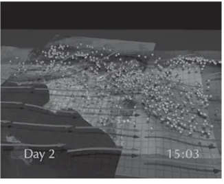
26.3.2.2 Point Creation Controlled by a Background Mesh
Another way to control the point spacing in the domain is to use a background mesh. A mesh is overlaid over the domain and at each node a point spacing is specified. To encompass this approach within the framework of Algorithm II, the point distribution functiondpfor a prospective point is obtained from the interpolated spacing from the background mesh. Within Algorithm II step 4b is replaced by the interpolation of dp from the background mesh. The effect is similar to that achieved by sources.
26.3.2.3 Boundary Integrity
followed here is an extension of earlier work and is closely related to the work of George. Both these approaches involve the addition of points toblockthe penetration of tetrahedra through the boundary surface. In the former approach, points were added on the boundary, which were then connected to the surrounding points using the Delaunay triangulation procedure. In two dimensions and in some cases in three dimensions, this approach proves to be adequate. Hence, the approach used in two dimensions uses this technique. However, in three dimensions, for some severe cases, it proves to be difficult to completely ensure the reconstruction of surface triangles. Hence, a different approach has been devised for three dimensions, which also involves the addition of points, but these are connected directly to the tetrahedral construction rather than using the Delaunay triangulation. A finite number of direct connections can be formulated for all types of tetrahedral penetration and hence in the proposed procedure the recovery of the surface can be guaranteed.
The necessary and sufficient conditions for a face with nodes (P,Q,R) to be present in the triangulation
{l},l =1,Tare as follows:
1. The nodesP, Q, andRexist in the tetrahedral construction{l},l =1,T.
2. The cyclic combinations ofP,Q, andRthat is,PQ, QR, RPoccur in one of the tetrahedra in the construction{l},l =1,T.
3. The combination (P,Q,R) exists in one of the tetrahedra in{l}, l =1,T.
Hence, to recover an arbitrary set of triangular faces, these three conditions must be met for each face. The first condition appears to be self-evident.
If a boundary face is not in, this is because edges and faces of the tetrahedra{}intersect the required face. Since a face is formed from edges, and it is assumed that the pointsP,Q and Rare present, it is necessary to firstly recover edgesPQ, QR, RPand then the face (P,Q,R). This is achieved, for a given face PQR,by firstly finding the tetrahedra which are intersected by the edgesPQ, QR,andRP. These tetrahedra are then modified and new tetrahedra created so that the required edges are present. Once edges are present, a similar procedure follows to recover the face. If the edgesPQ, QR,andRPexist but the face (P,Q,R) does not exist, then all tetrahedra which possess at least one edge which intersects the face (P,Q,R) are determined. These tetrahedra are then modified accordingly to recover the missing faces.
26.3.2.4 Edge Swapping
In circumstances where it is required to have a complete surface, although there is not a fixed constraint that a given set of faces is recovered, it is possible to ensure boundary faces are coincident with faces within the tetrahedral construction by swapping edges within the boundary surface triangulation. If in the tetrahedral construction facesABCandBCDexist, but in the surface triangulation facesACDandABD exist, then the two can be made to agree if in the surface triangulation edgeADis replaced byBC. There are conditions under which such a transformation is not allowed and these must be checked.
Edge swapping can be incorporated as an option. However, if it can be used, it can greatly reduce the amount of work to be carried out in the edge and face recovery routines.
26.3.2.5 Boundary Edge Recovery
The procedure to recover a missing edge of a boundary face involves two steps. First, it is necessary to identify the faces, edges, and points of tetrahedra which the edge intersects. Second, local transforma-tions involving tetrahedra are performed to recover the edge. The intersectransforma-tions of edges with tetrahedra can be readily computed. Once this has been performed, a set of transformations are used to recover edges.
26.3.2.6 Boundary Face Recovery
FIGURE 26.9 Volume grid of Ford Explorer.
FIGURE 26.10 Surface grid of Ford Explorer interior.
tetrahedra can penetrate the interior of a face but not the boundary face edges. If a boundary face is not present, it is necessary to determine all tetrahedra which intersect the face. One, two, three, or four edges and associated segments of a tetrahedra can intersect a face. Hence, for each missing face, all tetrahedra which have an edge or edges which intersect the face are determined and each of the tetrahedra are then classified accordingly.
26.3.2.7 Removal of Added Points
Most of the transformations used to recover the edges and faces in both 2-D and 3-D grids involve the creation of one or more points. These added surface points are used purely as part of the boundary recovery procedure and are removed after the boundary is complete. The mechanics of node removal involve taking each added point in turn and finding all elements connected to it. These elements are deleted leaving an empty polyhedron, which is then triangulated in a direct manner by finding point connections which lead to the optimum-shaped tetrahedral construction. This is a rapid process since this operation is performed locally for a relatively small number of points. A pictorial view of an unstructured grid for automotive application is presented inFigure 26.9 and Figure 26.10.The grid is generated by advancing front local reconnection algorithm [Marcum 1995].
26.3.3 Hybrid Grid Generation
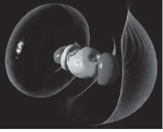
(a) (b)
FIGURE 26.11 Hybrid grid around a launch vehicle with boosters: (a) grid at an initial state and (b) grid after booster separation.
the sine of the minimum angle of the triangle. Therefore, to reduce the truncation error the number of triangles in the boundary layer has to increase and, consequently, it will increase the total number of cells in the field. This will lead to more memory and central processing unit (CPU) time for the flow solver. The structured grid in the boundary layer will help to overcome these difficulties.
The basic steps involved in hybrid grid generation are the following. The first step is to decompose the complex geometries into simple geometric entities. A structured grid is generated around these geometric entities using an advancing layer-type method based on the surface normals together with the application of a local elliptic solver [Koomullil et al. 1996a]. The second step involves the trimming of the overlapping structured grid from different solid bodies in the domain, by comparing the aspect ratio. Cells having aspect ratio less than unity are removed. In the third step the void in the physical domain after the trimming of the structured grid is filled with unstructured grid.
The hybrid grid for dynamic motion-type geometries can be generated quickly and efficiently using the approach present in Koomullil et al. [1996a]. An example of a hybrid grid for the moving geometry problem is illustrated inFigure 26.11.The strap-on separation from the main launch vehicle booster is shown in this figure. The relative position of the strap-ons and booster rockets at different times and the hybrid grid around this configuration is shown in Figures 26.11a and b.
26.3.3.1 Grid Adaption: Construction of Weight Functions
Application of the equidistribution law results in grid spacing inversely proportional to the weight function, and hence, the weight function determines the grid point distribution. Ideally, the weight would be the local truncation error ensuring a uniform distribution of error. Determination of this function is one of the most challenging areas of adaptive grid generation. The overall solution is only as accurate as the least accurate region. Thus, excessive resolution in certain regions does not increase the accuracy of the overall solution. Evaluation of higher order derivatives from discrete data is progressively less accurate and subject to noise. However, lower order derivatives must be nonzero in regions of wide variations of higher order derivatives, and are proportional to the rate of variation. Therefore, it is possible to employ lower order derivatives as a proxy for the truncation error.