Received November 22nd, 2011, Revised October 25th, 2012, Accepted for publication November 6th, 2012.
Copyright © 2012 Published by LPPM ITB,ISSN: 1978-3043, DOI: 10.5614/itbj.sci.2012.44.3.7
A Singular Perturbation Problem for Steady State
Conversion of Methane Oxidation in a Reverse Flow
Reactor
Aang Nuryaman1,3, Agus Yodi Gunawan1, Kuntjoro Adji Sidarto1 & Yogi Wibisono Budhi2
1
Industrial and Financial Mathematics Research Group,
Faculty of Mathematics and Natural Sciences, Institut Teknologi Bandung Jalan Ganesa 10 Bandung, Jawa Barat 40132, Indonesia
2
Design and Development Processing Research Group, Faculty of Industrial Technology, Institut Teknologi Bandung, Jalan Ganesa 10 Bandung,
Jawa Barat 40132, Indonesia
3
Department of Mathematics, Faculty of Mathematics and Natural Science Lampung University, Jl. Soemantri Brojonegoro 1, Gedong Meneng,
Bandarlampung 35145, Indonesia Email: [email protected]
Abstract. The governing equations describing methane oxidation in a reverse flow reactor are given by a set of convective-diffusion equations with a nonlinear reaction term, where temperature and methane conversion are dependent variables. In this study, the process is assumed to be a one-dimensional pseudo-homogeneous model and takes place with a certain reaction rate in which thewhole process ofthereactor is still workable. Thus, the reaction rate can proceed at a fixed temperature. Under these conditions, we can restrict ourselves to solving the equations for the conversion only. From the available data, it turns out that the ratio of the diffusion term to the reaction term is small. Hence, this ratio is considered as a small parameter in our model and this leads to a singular perturbation problem. Numerical difficulties will be found in the vicinity of a small parameter in front of a higher order term. Here, we present an analytical solutionby means of matched asymptotic expansions. The result shows that, up to and including the first order of approximation, the solution is in agreement with the exact and numerical solutions of the boundary value problem.
Keywords: asymptotic analysis; boundary layer; methane oxidation process; pseudo homogeneous; reverse flow reactor; steady state conversion.
1
Introduction
required to accelerate the conversion and normally preheating would be required to achieve optimal conversion conditions, however, by using the heat output from the reaction and appropriate cooling, preheating can be avoided and optimal chemical conversion conditions can be realized.
A concept successfully used in methane combustion is the catalytic reverse flow reactor (RFR). This concept was first discussed by Frank-Kamenetski [1] and was reviewed by Matros and Bunimovich [2]. An RFR is a packed-bed reactor in which the flow direction is periodically reversed totrap a hot zone within the reactor.
The common features of the combustion process in an RFR are usually the reaction-convection-diffusion equations with time-periodic coefficients and time-periodic boundary conditions. Garg, et al. [3] have observed that an adiabatic operation leads to periodic, period-1 symmetric states at which the temperature and concentrationprofiles at the beginning and end of a flow-reversal period are mirror images.
Earlier studies [4-10] mostly focused on the determination of the steady state temperature profile within the reactor. The simulation of Gosiewski and Warmuzinsky [5] showed that the heat recovery by hot gas withdrawal from the reactor guaranteed more favorable symmetry of the half-cycle-temperature profile. For a cooled RFR, Khinast and Luss [8] observed that if reactor cooling was increased, the symmetric temperature profile became unstable and either a periodic asymmetric, a quasi-periodic or a chaotic state was obtained. Salomon,
et al. [11] pointed out that the radial temperature gradient exists in both the inert and catalytic sections.
In this paper, we will discuss the steady state solution of the conversionof methane oxidation in an RFR in only one direction, from the left to the right end. We assume that the model is one-dimensional pseudo-homogeneous with small temperature variations and no heat loss. This leads to an equation in terms of the conversion variable only with an isothermal non linear reaction rate. For this case, the reaction can be considered to take place at a fixed temperature. Rescaling the variables, we obtain a dimensionless equation in which a small parameter is contained in the highest order of the equation,which leads to a singular perturbation problem. We solve the derived equation by using the matched asymptotic expansion method (see Holmes [12] orVerhulst [13]).
perturbation techniqueis presented to find the solution of steady state conversion. The conclusions are written in the last section.
2 Mathematical Model
In our study, we consider a cooled RFR described by a one-dimensionalpseudo-homogeneous model that is taken from van Noorden [14], (see the detailed explanation in the Appendix). In the steady state, namely
t
0
, the resulting conversion equation is given by
1
0, 0 1 ~' '' 6 7
5 K K x
K (1)
and boundary conditionsare
0
0, '
1 0' 6
5 K
K , (2)
where
2 2
''
dx d
and
dx d
' . The values of the parameters are given in the
Appendix.
Dividing both hand sides in (1) and (2) by
K
~
7, we obtain
1
0, 0 1' ' '
3
x
(3)
0
0, '
1 0 '2
(4)where
3
K
5/
K
7, and
O
1
. In the next section, we present an asymptotic solution for the system (3)-(4).3
Asymptotic Solution
For
0
, (3) has two linearly independent solutions.However for
0
, (3) becomes a singular perturbation problem since we have a reduced order of the equation. To find the (outer) solution, we replace
x
byy
0
x
y
1
x
...
,and get for
O
1
of (3)-(4) the following equations
0 0, '
1 0, 0
1y0 y0 y0 (5)
with the general solution
1
0
y
x
outer
It is clear that (6) cannot fulfill the left boundary condition in (4). Thus, we end up with a boundary layer problem. To find the inner solution, we assume that there is a boundary layer at
x
0
. Let
x . (7)Applying the chain rule, we have
d d dx
d d d dx
d d d dx d
2 2 2
1
,
1
. (8)
Subtitution of (7) and (8) in (3), yields
1
01 2 2 2
3
d d d
d
. (9)
Let a solution
of (9) bey0
x
y1
x ...
0
1
...,
0
Y
Y . (10)
Substituting the expansion in (10) into (9) we obtain
0 ...
- 1
0
...
1
0
...
02 2 2
3
Y Y
d d Y
d d
. (11)
The correct balancing in (11) occurs if
3
2
1
or1
0
, which implies that
2
or
1
. In case
2
we can write theO
1
boundary-layer equation0
0 2
0 2
d
dY d
Y d
for0
and
0 0
0'
0 Y
Y (12)
The general solution of this problem is
Ce DY0 , (13)
where C and D are arbitrary constants. The boundary condition in (12) gives
0
D
, thus (13) becomes
Ce
Y0 . (14)
In the second case,
1
, the boundary-layer Eq. (11) becomes
0 ...
-
0
...
1
0
...
02 2
Y Y
d d Y
d
d , (15)
and the boundary condition leads to
0 ...
0
0 ...
'
0 Y
Y
. (16)
The O
1 equation is given by
0 0, ;1 0 0
0
Y Y d dY
(17)
and the solution is
/ 0 1 1
x
e e
Y . (18)
Note that from the
O
1
equation for case
1
the matching process between the outer and the inner solutionsis automatically satisfied, i.e.Y
0
y
0
0
.Hence, the composite solution for
O
1
is
/
0 0
0 1 1
x
e y
Y x y
x . (19)
For
O
, from (3)-(4) we get the outer solution isy
1
x
0
and from (15)-(16) the boundary layer equation is
0
0, ;
1 '
0 1 / 2 1
1 Y e Y Y
d
dY
where the solution is given by
e e
Y1 13 12 . (20)
Again, the matching process for
O
is automatically satisfied and then the composite solution is the inner solutionY
1
, as in (20). So the asymptotic solution for our problem up to and includingO
is
... 1
1
1 / 3 2
x e x e e .or
... 1
1 / 3 / 2 /
x x xe xe
e
In comparison, the exact general solution of (3) is
rx rxBe Ae
x 1 1 2
. (22)with 2 4 2 2 1
r and 2
2 2 2 4 r .
If we expand 24at
0
until three terms and apply the boundary conditions (4), we get3 2 2 2 2 3 2 2 2 3 2 2 3 2
e e e A and 3 2 3 2 2 3 2 2 2 3 2 2 3 2 e e e BThe three term expansion of
24
is considered since the rootsr
1andr
2 in(22) contain a factor 1/2
2. For a small
, we note that
2 2
e is smaller than any power of
as
0
. Thus, for
0
we get A tends to zero and Btends to –1. Hence, we can rewrite (22) as
x e ESTx 2 3 5 2 3 2 ... 4 2 2 1
.
e
e
EST
x x
13 25 ...
1
. (23)
where EST stands for exponentially small terms. In deriving the expansion (21),
we expand
x
e
2 ...
1
5
3
for x near the origin, so we get (23), as follows
1 e 1 13 25 ... x ...
... 2
1 3 5
x x
x
e e
x
e . (24)
which is in agreement with (22), except for factor
2
/
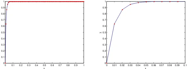
5 in the fourth term.Plots of the asymptotic solution and the exact and the numerical solution of (3)-(4) for
0
.
05
and
0
.
005
and
2are shown in Figure 1 and Figure 2. The numerical solutions of (3)-(4) are obtained by using the toolbox for boundary value problems in MATLAB.Figure 1 Left: Plot
of methane conversion as a function of position x, for05
.
0
where the dashed line represents the exact solution and the solid line represents the asymptotic solution. The dotted symbol represents the numerical solution. Right: the zoom of
for a small window of x.Figure 2 Left: Plot
of methane conversion as a function of position x, for005
.
0
where the dashed line represents the exact solution and the solid line represents the asymptotic solution. The dotted symbol represents the numerical solution. Right: the zoom of
for a small window of x.0 0.1 0.2 0.3 0.4 0.5 0.6 0.7 0.8 0.9 1 0
0.1 0.2 0.3 0.4 0.5 0.6 0.7 0.8 0.9 1
x
0 0.01 0.02 0.03 0.04 0.05 0.06 0.07 0.08 0.09 0.1 0
0.1 0.2 0.3 0.4 0.5 0.6
x
0 0.1 0.2 0.3 0.4 0.5 0.6 0.7 0.8 0.9 1 0
0.1 0.2 0.3 0.4 0.5 0.6 0.7 0.8 0.9 1
x
0 0.01 0.02 0.03 0.04 0.05 0.06 0.07 0.08 0.09 0.1 0
0.1 0.2 0.3 0.4 0.5 0.6 0.7 0.8 0.9 1
x
We observe that the results of the asymptotic solution and the numerical simulations hardly differ. The effect of reducing the magnitude of
is to shorten the window of the rapid changes of the solution.4
Conclusion
Based on available data, we constructed a singular perturbation problem for the steady state conversion of the methane oxidation process in a reverse flow reactor. The small parameter in our problem occurred both in front of the convective and diffusive terms in which the order of the diffusive term is higher than the convective one. Also, one of the boundary conditions had an order between the orderof those terms. Using the matched asymptotic expansion method and assuming that the boundary layer occurs at
x
0
, we solved the equation up to and including the first-order approximation. The present asymptotic solution was quite in agreement with the numerical solution and the exact solution.Acknowledgements
The authors would like to thank the reviewers for their invaluable suggestions and corrections. This research was supported by Program Riset dan Inovasi KK ITB 2011 with grant no. 215/I.1.C01/PL/2011.
References
[1] Frank-Kamenetskii, D.A., Diffusion and Heat Transfer in Chemical Kinetics, Princeton Univ. Press, Princeton, NJ, 1955.
[2] Matros, Yu. Sh., & Bunimovich, G.A., Reverse-Flow Operation In Fixed Bed Catalytic Reactors, Catalysis Reviews: Science & Engineering, 38, pp. 1-68, 1996.
[3] Garg, L., Luss, D., & Khinast, J.G., Dynamic and Steady-State Features of a Cooled Countercurrent Flow Reactor, AIChE Journal, 46(10), pp. 2030-2040, 2000.
[4] Gosiewski, K., Effective Approach to Cyclic Steady State in the Catalytic
Reverse-Flow Combustion of Methane, Chemical Engineering Science,
59, pp. 4095-4101, 2004.
[5] Gosiewski, K. & Warmuzinsky, K., Effect of the Mode of Heat Withdrawal on the Asymmetry of Temperature Profiles in Reverse-Flowreactors, Catalytic Combustion of Methane as A Test Case, Chem. Eng. Sci., 62(10), pp. 2679-2689, 2007.
[7] Khinast, J., Jeong, Y.O. & Luss, D., Dependence of Cooled Reverse-Flow Reactor Dynamics on Reactor Model, A.I.Ch.E. Journal, 45, pp. 299-309, 1999.
[8] Khinast, J. & Luss, D., Efficient Bifurcation Analysis of Periodically-Forced Distributed Parameter System, Computers and Chemical Engineering, 24, pp. 139-152, 2000.
[9] Salinger, A.G. & Eigenberger, G., The Direct Calculations of Periodic States of The Reverse Flow Reactor-I, Methodology and Propane Combustion Results, Chemical Engineering Science, 51, pp. 4903-4913, 1996.
[10] Salinger, A.G. & Eigenberger, G., TheDirect Calculations of Periodic States of The Reverse Flow Reactor-II. Multiplicity and Satability. Chemical Engineering Science, 51, pp. 4915-4922, 1996.
[11] Salomons, S., Hayes, R.E., Poirier, M. & Sapoundjiev, H., Modelling a Reverse Flow Reactor for The Catalytic Combustion of Fugitive Methane Emission, Computer and Chemical Engineering, 28, pp. 1599-1610, 2004.
[12] Holmes, M.H., Introduction to Perturbation Methods, Texts in Applied Mathematics, 20, Springer-Verlag, New York, 1998.
[13] Verhulst, F., Methods and Applications of Singular Perturbations, Texts in Applied Mathematics, 50, Springer-Verlag, New York, 2000.
[14] Van Noorden, T.L., Verduyn Lunel, S.M.V. & Bliek, A., The Efficient Computation of Periodic States of Cyclically Operated Chemical Processes, IMA Journal of Applied Mathematics, 68, pp. 149-166, 2003.
Appendix
In the RFR, a 1-D pseudo-homogeneous model is governed by a set of the following equations
1 2 3 1 4 1 0, 0,1
t K xx K x K g K x
(25)
5 6 7
1
0,
0
t
K
xxK
xK g
t
, (26)
5 5
1.6656 10 exp 25.785 1 / 1.6656 10 exp 25.785 /
g
,
where
x
,
t
,
x
,
t
are dimensionless variables for temperature and conversion, respectively, Kj are dimensionless parameters, for j1,2,...,7,containing the entry point, the boundary conditions for flow in the right direction are
1 x
0,
20,
1 ,
K
t
K
t
K
5
x
0,
t
K
6
0,
t
(27)
1,
1,
0
x
t
xt
(28)These two boundary conditions are known as Danckwert’s boundary conditions.
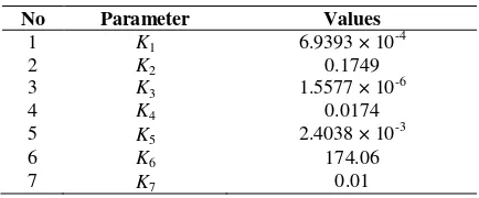
Table 1 The dimensionless parameter values of RFR.
No Parameter Values
1 K1 6.9393 × 10⁻⁴
2 K2 0.1749
3 K3 1.5577 × 10⁻⁶
4 K4 0.0174
5 K5 2.4038 × 10
-3
6 K6 174.06
7 K7 0.01
Under assumptions steady state condition and
g
was evaluated at certain temperature
* in which the processs can still be handled by the reactor, the value of temperature state in this condition may be considered as constant. Hence, we can eliminate the energy transfer equation from the process. To see the behavior ofK
~
7
K
7g
* , we plotg
as a function of
, as shown in Figure 3. Based on this plot, we approximateK
~
7
2
.
5
10
4.Figure 3 Plot
vsg
.1 1.5 2 2.5 3 3.5
0 0.5 1 1.5 2 2.5
3x 10 6
g(