International Review of Economics and Finance 9 (2000) 157–179
Short-term eurocurrency rate behavior and
specifications of cointegrating processes
Thomas C. Chiang*, Doseong Kim
Drexel University, Department of Finance, 32nd & Chestnut Streets, Philadelphia, PA 19104, USA Received 21 July 1998; accepted 1 April 1999
Abstract
This article presents empirical evidence on short-term behavior based on seven Eurocurrency market rates. Empirical analysis suggests that there is two-dimensional cointegration. First, the domestic short-term interest rate is cointegrated with longer-term interest rates within a particular country. Second, the domestic short-term interest rate is cointegrated with the comparable foreign short-term interest rate adjusted for the foreign exchange forward premium (discount). The empirical evidence confirms that an error-correction model combining both dimensional market-correcting processes better explains short-term interest rate movements.
2000 Elsevier Science Inc. All rights reserved.
JEL classification:E43; F3
Keywords:Eurocurrency rate; Error correction model; Term structure of interest rates; J-test
1. Introduction
Recent advances in time-series analysis and cointegration tests on interest rate series suggest that interest rates tend to follow some common stochastic factors (Choi & Wohar, 1991; Mougoue, 1992; Engsted & Tanggaard, 1994). Focusing on the term structure of interest rates, it has been shown that short- and long-term interest rates are cointegrated within a particular country (Arshanapalli & Doukas, 1994; Chiang & Chiang, 1995). An important implication of this finding is that the lagged error correc-tion term obtained from the long-term equilibrium equacorrec-tion implied by the term– structure relationship can be used to predict the subsequent changes of the short-term interest rates.
However, evidence has been found that short-term interest rates with the same
* Corresponding author. Tel. 215-895-1745, 609-265-1315; fax: 609-265-0141. E-mail address: [email protected] (T.C. Chiang)
maturities across different countries are also cointegrated (Mougoue, 1992), especially for a small open economy. This means that the error-correcting term obtained from the lagged covered-arbitrage margin can be used to predict future changes of short-term interest rates.
An important message obtained from these cointegration analyses is that it would be more informative if interest rate behavior could be modeled in an error-correcting process since this representation contains both levels and differences of explanatory variables concerned. Kugler (1990), Choi and Wohar (1991), Bradley and Lumpkin (1992), Mougoue (1992), Arshanaplli and Doukas (1994), and Chiang and Chiang (1995) present evidence to support the specification of the error-correction model (ECM). Yet in examining these two dimensions of cointegration, it is natural to ask which dimension of the equilibrium relationship is more relevant in an integrated international market. Are these two error-correcting terms substitutable or comple-mentary to each other? Concrete empirical evidence on this issue would provide more insight into the nature of cointegration. As a result, the findings could offer an empirical basis for specifying the error-correcting model in predicting interest rate movements. In this article, we consider two theoretical frameworks—the term-structure relation-ship of interest rates and the international interest rate parity condition—for guiding the structural relationship between the short-term interest rate and its equilibrium level. As the model stands, the existence of these long-run structural relationships will translate into a framework of cointegrated processes. The article is organized as follows. Section 2 provides a general discussion of the properties of cointegration and a description of the error-correction representations. Section 3 discusses the data and the evidence of unit roots and cointegration tests. Section 4 reports and discusses the empirical results for different specifications of the error-correction models for the Euro-interest rates. Section 5 contains concluding remarks.
2. Cointegrating factors and error correction models
To illustrate the tenet of the error-correction model (Muscatelli & Jurn, 1992), let
us consider two time series, {yt} and {zt}, which are first-difference stationary, that is,
integrated of order 1, I(1). It is generally true that any linear combination of these two series is also I(1). However, if there is a linear combination of these two series
such that ut 5 yt 2 b0 2 b1zt is stationary, I(0), then {yt} and {zt} are said to be
cointegrated.
By applying this notion to describe short-term Eurocurrency rate (rt) behavior, it
is necessary to identify the equilibrium rate in which the cointegrating equation is being specified. Two candidate variables may be considered. The first is the
long-term rate (Rt) within a given currency rate; the second is the effective foreign interest
rate (r*ft), which is defined as the Eurodollar deposit rate (r*t) with the same maturity
plus the U.S. dollar forward premium (Boothe, 1991). In the following sections, we shall provide a brief economic justification for using these rates.
usually referred to as the long-term interest rate. As stated by the expectations theory of the maturity structure of interest rates, the long-term interest rate is a weighted average of current and expected short-term interest rates. Thus, we can write a long-run relationship between short rate and long rate as
rt5b10 1b11Rt1u1,t, (1)
whereb10and b11are estimated parameters,rtis the short-term interest rate,Rtis the
long-term interest rate, and u1,t is an error term. Expressing Eq. (1) in a short-run
dynamic process, we write an error-correction model (ECM) as
Drt5C11
o
operator, andu1,t21is the error-correction term obtained from the long-run equilibrium
equation. This term reflects the fact that the short-term interest rate is in a state of disequilibrium that would be revised, moving toward its long-run level. To differentiate our model specifications, we shall call Eq. (2) a domestic term-structure ECM specifica-tion (Hall, et al., 1992; Nourzad & Grennier, 1995).
Notice that the specification of Eq. (2) gives no consideration to the effect derived from foreign markets. It has been observed that, for a small open economy, the short-term interest rate cannot deviate significantly from the comparable global level of interest rates. Thus, it can be argued that the Canadian and other short-term Eurocur-rency rates will maintain a close relationship with Eurodollar rates having the same level of maturity. This tight relationship may stem from institutional arrangements in a global setting or from monetary policy coordination among national central banks (Mougoue, 1992).
It should be noted that the interest rate differentials do not provide all the explana-tion to describe internaexplana-tional capital movements. To compare short-run investment returns across national borders, it is necessary to take into account the exchange-rate factor. As described by the international interest rate parity condition, the domestic
short-term interest rate (rt) should not deviate significantly from the comparable
foreign short-term interest rate adjusted by a forward premium or forward discount
on the foreign currency (r*ft). Thus, we can write a long-run relationship between rt
and rft* as
rt5b20 1b21 rft*1 u2,t, (3)
whereb20andb21are estimated parameters. Theu2,tin Eq. (3) is an error term, which
may capture the information in relation to deviations from covered interest rate parity (CIP) resulting from real world frictions, transactions costs, currency preference, or different speeds of market reaction (Abeysekera & Turtle, 1995; Atkins, 1993; Bhatti & Moosa, 1995; Cody, 1990; Committeri et al., 1993). This information plays an important role in explaining international arbitrages, which in turn affect short-term interest
rate movements. A short-run ECM for describing the relationship between rt and
Drt5C21
o
m
j50
g2jDr*f,t2j1
o
nj51
p2jDrt2j2 c2u2,t211 e2,t, (4)
whereC2,g2,p2, andc2are estimated parameters,rft* is the effective foreign investment
return (Eurodollar rate plus a forward exchange premium on the U.S. dollar); rt is
the domestic investment return (Canadian and other Eurocurrency rates) of a given
maturity; and e2,t is an error term. Although no particular argument in Eq. (4) has
been used to describe the source that causes deviations from CIP, the inclusion of
the u2,t21 term allows us to use additional information to predict future short-term
interest rate movements. Of course, this econometric treatment is subject to empirical verification.
3. Data and unit-root and cointegration tests
3.1. Data
In this study, we employ weekly data of Eurocurrency deposit rates and spot and
forward exchange rates for the period from June 1, 1973, through August 2, 1996.1
The Eurocurrency rate data set includes 1-, 3-, 6-, and 12-month rates for Eurocurrency deposits denominated in British pounds (BP), Canadian dollars (CD), German marks (GM), Italian lira (IL), Japanese yen (JY), Swiss francs (SF), and U.S. dollars. The Eurocurrency rates are bid rates at the close of trading in London. The foreign exchange rate data contain spot exchange rates and 1-, 3-, 6-, and 12-month forward exchange rates of BP, CD, GM, IL, JY, and SF. The foreign exchange rates are defined as units of foreign currencies per U.S. dollar. All Eurocurrency rate and foreign exchange rate data are measured at the end of the week, as obtained from Data Resources, Inc.
3.2. Unit-Root Tests
To estimate short-run dynamic equations, researchers usually begin with testing the stationarity of the series under consideration. To this end, we employ the Dickey Fuller (DF) (1979) and augmented Dickey Fuller (ADF) (1981) tests to examine whether the time-series variables are stationary or not. Table 1A reports results of unit-root tests for 1-, 3-, 6-, and 12-month Eurocurrency deposit rates. The test statistics indicate that, with the exception of the 1-month rate for the SF, the null hypothesis of a unit-root cannot be rejected for the levels of Eurocurrency rates. However, the null hypothesis is rejected for all cases when Eurocurrency rates are first differenced. This means that, in general, the levels of Eurocurrency rates are nonstationary while the first differences are stationary. These results are consistent with the findings of Kugler (1990), Mougoue (1992), Arshanapalli and Doukas (1994), and Chiang and
Chiang (1995).2
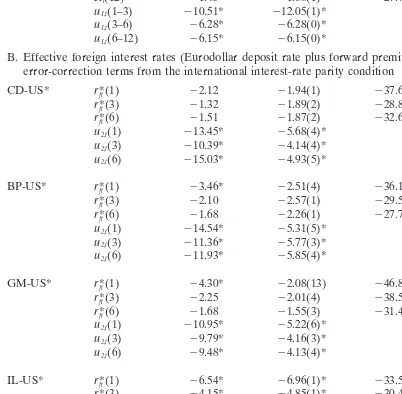
Table 1B reports the results of unit-root tests for 1-, 3-, 6-, and 12-month foreign
investment returns,r*ft, which are defined as Eurodollar deposit rates (Euromark for
Table 1
Unit-root and cointegration tests
Level First Differencing
Currency Variables DF ADF(Lags) DF ADF(Lags)
A. Eurocurrency rates and error-correction terms from the term-structure relation
Table 1 (Continued)
Level First Differencing
Currency Variables DF ADF(Lags) DF ADF(Lags)
SF rt(1) 22.98** 22.87(5)** 231.74* 217.31(4)*
rt(3) 22.01 22.35(1) 228.98* 228.98(0)*
rt(6) 21.67 22.15(2) 227.97* 220.73(1)*
Rt(12) 21.45 21.88(1) 227.73* 227.73(0)*
u1,t(1–3) 210.51* 212.05(1)*
u1,t(3–6) 26.28* 26.28(0)*
u1,t(6–12) 26.15* 26.15(0)*
B. Effective foreign interest rates (Eurodollar deposit rate plus forward premium on U.S. dollar) and error-correction terms from the international interest-rate parity condition
CD-US* r*ft(1) 22.12 21.94(1) 237.64* 237.64(0)*
r*ft(3) 21.32 21.89(2) 228.80* 228.80(0)*
r*ft(6) 21.51 21.87(2) 232.66* 221.69(1)*
u2,t(1) 213.45* 25.68(4)*
u2,t(3) 210.39* 24.14(4)*
u2,t(6) 215.03* 24.93(5)*
BP-US* r*ft(1) 23.46* 22.51(4) 236.10* 220.47(3)*
r*ft(3) 22.10 22.57(1) 229.51* 223.59(1)*
r*ft(6) 21.68 22.26(1) 227.78* 227.78(0)*
u2,t(1) 214.54* 25.31(5)*
u2,t(3) 211.36* 25.77(3)*
u2,t(6) 211.93* 25.85(4)*
GM-US* r*ft(1) 24.30* 22.08(13) 246.84* 211.42(12)*
r*ft(3) 22.25 22.01(4) 238.56* 216.47(3)*
r*ft(6) 21.68 21.55(3) 231.40* 219.99(2)*
u2,t(1) 210.95* 25.22(6)*
u2,t(3) 29.79* 24.16(3)*
u2,t(6) 29.48* 24.13(4)*
IL-US* r*ft(1) 26.54* 26.96(1)* 233.56* 219.19(4)*
r*ft(3) 24.15* 24.85(1)* 230.40* 225.71(1)*
r*ft(6) 22.86** 23.25(2)** 229.36* 223.89(1)*
u2,t(1) 26.57* 26.57(0)*
u2,t(3) 26.10* 25.36(6)*
u2,t(6) 27.94* 26.68(1)*
JY-US* r*ft(1) 29.26* 26.26(7)* 235.21* 221.08(8)*
r*ft(3) 24.92* 24.47(5)* 235.65* 216.12(5)*
r*ft(6) 23.63* 24.07(4)* 233.79* 214.27(4)*
u2,t(1) 217.94* 27.80(3)*
u2,t(3) 23.77** 21.63(1)
u2,t(6) 22.42 20.93(1)
Table 1 (Continued)
Level First Differencing
Currency Variables DF ADF(Lags) DF ADF(Lags)
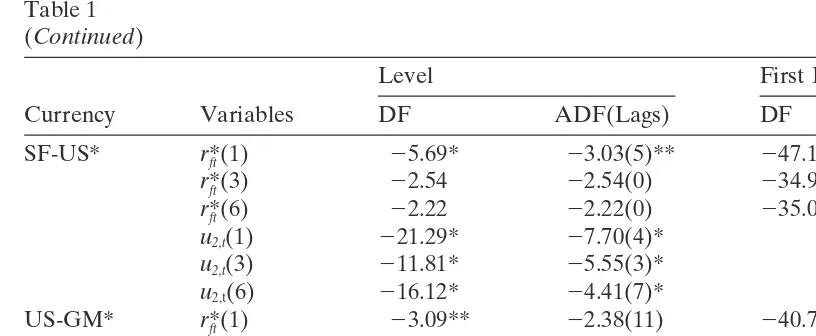
SF-US* r*ft(1) 25.69* 23.03(5)** 247.11* 219.76(4)*
For domestic interest rates and effective foreign interest rates, the regression model for the Dickey-Fuller (DF) test isDxt5 a 1 rxt211 et, wherext: {rtandRt} (domestic interest rates) or {rt} (effective
foreign interest rates defined as Eurodollar rates plus forward exchange premium on U.S. dollar) for testing H0:r 50. The augmented Dickey-Fuller (ADF) test is given byDxt5 a 1 rxt211
o
ki51giDxt2i1et. The numbers in the parentheses are the optimal lag lengths for the ADF test. The choice of optimal
lag length (k) for the ADF test is determined by adding an additional lag until the joint significance (the Ljung-Box Q-test) of the residual autocorrelation up to the 8th order is rejected at a 5% significance level. The * and ** indicate statistical significance at the 1% and 5% levels, respectively. The critical values for the 1% and 5% significance levels are23.43 and22.86, respectively (Fuller, 1976).
Effective foreign interest rates,r*ft, which domestic investors can obtain from investment in Eurodollar
deposit rates, plus currencies’ forward premiums,ft2st, on the U.S. dollar based on the covered
Interest-Rate Parity. That is,r*ft 5r*t 1(ft2st), wherer*ft 5effective foreign interest rates from Eurodollar (or
Euromark) deposit rates;r*t 5Eurodollar (or Euromark) rates;ft5forward exchange rate in the natural
log; andst5spot exchange rate in the natural log. In the cases of Canada, Japan, and European countries,
we assume that the United States is the foreign country. For the United States, effective foreign interest rates are constructed as Euromark deposit rates plus forward premiums on the German mark. Germany is assumed to be the foreign country.
Error correction terms,u1,t, are obtained from a cointegrating equation ofu1,t5rt2b102b11Rt, where
rtis the short rate andRtis the adjacent longer rate. Error correction terms,u2,t, are obtained from a
cointegrating equation ofu2,t5rt2b202b21r*ft. The DF tests for cointegration are based on the regression
equation ofDui,t5 riui,t211 ei,t. The ADF tests for cointegration are based on the regression equation
ofDui,t5 riui,t211 Skj52gijui,t2j1 ei,t. For DF and ADF tests for cointegration, the critical values are24.07
(23.77) and23.37 (23.17) at the 1% and 5% significance levels, respectively (Engle & Granger, 1987). The choice of optimal lag length (k) for the ADF test is determined by adding additional lag until the joint significance (Ljung-Box Q-test) of residual autocorrelation up to the 8th order is rejected at the 5% level of significance.
(forward premium on the German mark for U.S. investors). With the exceptions of the JY and IL, the evidence shows that the null hypothesis cannot be rejected for the
interest rate levels. Yet, for the first differences of ther*ft series, the null hypothesis
We also examine the results of the error terms on the long-run equilibrium Eqs. (1) and (3). Evidence shows that for virtually all of the residual series, the null
hypothesis of unit roots is rejected. Specifically, theu1,t’s shown in Table 1A indicate
that these values are highly significant. This suggests that two adjacent interest rates are cointegrated across the entire term-structure spectrum.
To examine the international market cointegration hypothesis, we examine the
relationship between the domestic interest rate (rt) and the foreign interest rate
ad-justed by the exchange rate factor (r*ft). The stationarity tests of the residuals derived
from the cointegrating Eq. (3) are presented in Table 1B. For all cases except JY for 3-, 6-, and 12-month maturities, DF and ADF tests on the residuals from equilibrium regressions show that those residuals are stationary at the one percent significance level. This suggests that cointegration between domestic and foreign interest rates
adjusted by a forward premium (discount) is confirmed by the data.3
4. Estimation of error-correction models
Having performed the cointegration tests, we are ready to apply the two-step procedure proposed by Engle and Granger (1987). In the first step, the long-run relationship (the level of the variables) is estimated by OLS regressions. In the second step, the short-run dynamic (the change of the variables) is estimated by including a lagged error term from the long-run relationship regression. This two-step procedure requires that all the variables in the error correction model regressions are stationary, otherwise OLS estimates are inappropriate (West, 1988; Mehra, 1993). To estimate the error-correction model, the optimal lag length of independent variables has to be determined. Because most Eurocurrency rates and exchange rates are highly sensitive and efficient and also for the purpose of comparison across countries and maturities, we employ the first-order lag for independent variables. The estimated results for these two specifications of ECM representations (Eqs. [2] and [4]) are presented in
Tables 2 and 3.4,5
4.1. Evidence from domestic term-structure ECM
The findings shown in Table 2 on the relationship between short rates and long rates for a given currency are consistent with those presented by Chiang and Chiang (1995), who used monthly short-end Eurocurrency rates. First, all estimated equations
have a relatively high R2, ranging from 0.65 to 0.93. The DW statistics indicate the
absence of first-order serial correlation.
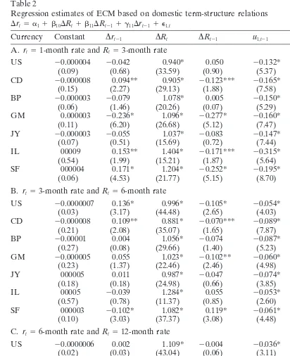
Table 2
Regression estimates of ECM based on domestic term-structure relations Drt5 a11 b10DRt1 b11DRt211 g11Drt211 e1,t
Currency Constant Drt21 DRt DRt21 u1,t21 R2 SEE DW
A. rt51-month rate andRt53-month rate
US 20.000004 20.042 0.940* 0.050 20.132* 0.80 0.0014 1.99
(0.09) (0.68) (33.59) (0.90) (5.37)
CD 20.000008 0.094** 0.905* 20.123*** 20.165* 0.77 0.0014 2.00
(0.15) (2.27) (29.13) (1.88) (7.58)
BP 20.000003 20.079 1.078* 0.005 20.150* 0.79 0.0019 2.04
(0.06) (1.46) (20.26) (0.07) (5.29)
GM 0.000003 20.236* 1.096* 20.277* 20.160* 0.80 0.0010 1.95
(0.11) (6.20) (26.68) (5.12) (7.47)
JY 20.000003 20.055 1.037* 20.083 20.147* 0.65 0.0015 1.73
(0.07) (0.51) (15.69) (0.72) (7.44)
IL 00009 0.153** 1.404* 20.171*** 20.315* 0.83 0.0040 1.95
(0.54) (1.99) (15.21) (1.87) (5.64)
SF 000004 0.171* 1.204* 20.252* 20.195* 0.73 0.0020 1.97
(0.06) (4.53) (21.77) (5.15) (8.70)
B. rt53-month rate andRt56-month rate
US 20.0000007 0.136* 0.996* 20.105* 20.054* 0.93 0.0008 1.99
(0.03) (3.17) (44.48) (2.65) (4.03)
CD 20.000008 0.109** 0.881* 20.070*** 20.089* 0.83 0.0011 2.02
(0.21) (2.08) (35.07) (1.65) (7.87)
BP 20.00001 0.004 1.056* 20.074 20.087* 0.85 0.0014 2.01
(0.27) (0.08) (29.66) (1.40) (5.23)
GM 20.000005 0.055 1.023* 20.102** 20.060* 0.84 0.0007 2.00
(0.23) (1.37) (22.46) (2.46) (4.98)
JY 000005 0.011 0.987* 20.047 20.074* 0.80 0.0009 1.99
(0.18) (0.18) (24.98) (0.66) (3.85)
IL 00005 20.039 1.284* 0.055 20.053* 0.80 0.0027 1.99
(0.57) (0.78) (11.37) (0.85) (2.60)
SF 000003 20.102* 1.082* 0.119* 20.061* 0.83 0.0010 2.01
(0.10) (3.03) (37.37) (3.08) (4.48)
C. rt56-month rate andRt512-month rate
US 20.0000006 0.002 1.109* 20.004 20.036* 0.91 0.0009 1.99
(0.02) (0.03) (43.04) (0.06) (3.11)
CD 20.00001 20.112** 0.957* 0.114** 20.063* 0.86 0.0010 2.02
(0.34) (2.41) (38.85) (2.35) (4.34)
BP 20.00001 20.095* 1.071* 0.055 20.061* 0.86 0.0012 2.02
(0.32) (2.67) (39.85) (1.33) (4.53)
GM 20.000003 0.003 1.006* 0.010 20.034* 0.82 0.0007 1.99
(0.16) (0.09) (31.83) (0.28) (3.85)
JY 0.000007 0.033 1.059* 20.049 20.069* 0.78 0.0009 1.96
(0.27) (0.55) (22.39) (0.73) (3.48)
IL 20.000009 0.095*** 0.906* 0.001 20.116* 0.67 0.0023 1.93
(0.11) (1.67) (15.89) (0.01) (3.04)
SF 20.000002 20.008 1.072* 0.022 20.062* 0.83 0.0009 2.00
(0.08) (0.19) (38.58) (0.41) (4.34)
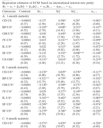
Table 3
Regression estimates of ECM based on international interest-rate parity
Drt5 a21 b20Dr*ft 1 b21Dr*ft211 g21Drt212 c2u2,t211 e2,t
Currencies Constant Drt21 Dr*ft Dr*ft21 u2,t21 R2 SEE DW A. 1-month maturity
CD-US 20.00002 20.157 0.580* 0.267 20.082* 0.66 0.0016 2.14
(0.37) (2.94) (11.09) (6.26) (3.06)
BP-US* 20.00003 20.185* 0.608* 0.215* 20.147* 0.72 0.0023 2.12
(0.52) (2.70) (14.41) (3.04) (4.11)
GM-US* 20.00002 0.016 0.449* 0.164* 20.056* 0.56 0.0015 2.02
(0.42) (1.48) (7.94) (7.94) (3.84)
JY-US* 0.00001 0.015 0.231** 0.071*** 20.099* 0.26 0.0022 2.01
(0.07) (0.18) (2.28) (1.67) (3.24)
IL-US* 20.00002 0.022 0.515* 0.005 20.072*** 0.59 0.0062 1.99
(0.12) (0.28) (9.62) (0.08) (1.68)
SF-US* 20.00003 20.132 0.332* 0.098*** 20.146* 0.36 0.0030 2.05
(0.39) (0.15) (2.75) (1.72) (4.11)
US-GM* 20.00001 20.151* 0.614* 0.147* 20.219* 0.70 0.0017 2.02
(0.28) (4.48) (13.21) (6.38) (9.34)
B. 3-month maturity
CD-US* 20.00001 20.235* 0.829* 0.276* 20.117* 0.84 0.0011 2.16
(0.24) (6.86) (16.76) (8.88) (4.27)
BP-US* 20.00001 20.321** 0.759* 0.340* 20.102* 0.83 0.0014 2.18
(0.23) (12.75) (33.46) (13.77) (4.13)
GM-US* 20.00001 20.136* 0.589* 0.271* 20.043* 0.66 0.0010 2.11
(0.43) (2.89) (9.79) (10.07) (3.07)
JY-US* 20.00003 0.029 0.377* 0.199** 20.004 0.46 0.0016 2.06
(0.74) (0.28) (3.55) (2.34) (0.51)
IL-US* 20.00003 0.163** 0.463* 20.019 20.069*** 0.47 0.0043 1.98
(0.25) (2.42) (9.52) (0.39) (1.66)
SF-US* 20.00002 20.209* 0.634* 0.268* 20.074* 0.65 0.0016 2.12
(0.35) (3.38) (7.27) (7.04) (3.21)
SF-US* 20.00001 20.279* 0.780* 0.268* 20.230* 0.86 0.0011 2.13
(0.26) (6.55) (23.61) (8.13) (6.77)
C. 6-month maturity
CD-US* 20.00001 20.273* 0.829* 0.330* 20.226* 0.82 0.0011 2.15
(0.19) (5.38) (19.67) (6.32) (4.40)
BP-US* 0.00000 20.301* 0.818* 0.348* 20.122* 0.88 0.0011 2.15
(0.01) (7.42) (51.47) (9.05) (5.59)
GM-US* 20.00001 20.018** 0.711* 0.237* 20.067* 0.76 0.0008 2.10
(0.27) (2.34) (18.56) (6.47) (3.92)
JY-US* 20.00003 479 0.406* 0.174*** 20.003 0.45 0.0014 2.03
(0.91) (0.38) (3.23) (1.75) (0.45)
IL-US* 20.00003 069 0.476* 0.055 20.098** 0.50 0.0029 1.97
(0.40) (0.81) (10.14) (1.07) (2.32)
SF-US* 20.00002 20.098 0.583* 0.215* 20.138* 0.62 0.0014 2.09
(0.36) (1.64) (8.05) (5.45) (5.12)
US-GM* 20.00001 20.205* 0.864* 0.207* 20.227* 0.92 0.0008 2.09
(0.25) (4.17) (49.84) (4.75) (5.66)
the long rate. In addition, the coefficients of the error-correction term in the ECM for shorter maturities are, in general, larger than those derived from longer maturities. This means that the adjustment speed is faster in the 1- and 3-month equations than in the 3- and 6-month equations, and it is faster in the 3- and 6-month equations than
in the 6- and 12-month equations.6
Third, all the contemporaneous terms of the change of the longer-term interest rates have a positive sign and are significantly different from 0 at the one percent level. This finding suggests that the short rate and the long rate are cointegrated in the short-run as well as in the long-run relationship. In addition, lagged long-term rates have an effect on the changes in short rates in some cases, even though the explanatory power is relatively weaker than the contemporaneous term. Thus, the evidence suggests that the long rate plays an important role in explaining the move-ments of the short-term interest rate.
Fourth, the coefficients on the lagged short-term interest rates appear to have mixed signs, depending on the country or maturity. The evidence did not indicate whether the interest rate series on the weekly base is in the nature of an extrapolative or a distributed lag process. Since the explanatory power is dominated by the change of the long rate and by the error-correction term, the lagged change in the short rate appear to be less significant.
4.2. Evidence from international interest rate parity ECM
The estimates of dynamic adjustments for international integrated capital markets are presented in Table 3. The findings are summarized as follows. First, the model
appears to have good explanatory power. TheR2for the estimated equations ranges
from 0.26 to 0.88, although these values are lower than in the previous model. The DW statistics indicate no first-order serial correlation.
Second, consistent with our earlier cointegration tests, all the error correction terms, with the exceptions of JY rates in the 3-, 6-, and 12-month cases, are highly significant. The negative sign of the error-correcting term implies that when there is a discrepancy between domestic and effective foreign returns, international arbitrage takes place, forcing Eurocurrency rates to revert to their long-run equilibrium level.
Third, changes in the effective Eurodollar rates have a positive sign and are highly significant. This finding suggests that Eurocurrency rates and effective Eurodollar rates have a tendency of co-movement, both in the short-run dynamic relationship as well as in the long-run equilibrium relationship. However, the significance of the lagged effective Eurodollar rates and the error-correcting terms suggests that the international interest rate parity condition does not necessarily hold true in an instanta-neous case.
5. Specification tests
Estimates of ECM indicate that both longer-term Eurocurrency rates of a given currency and effective foreign interest rates (Eurodollar rate plus a forward premium) for a given maturity have significant explanatory power. Moreover, both error-correct-ing terms contain significant information, which can be used to predict the short-end Eurocurrency rates. Apparently, the Eurocurrency market undergoes two-dimensional market arbitrage: intertemporal and spatial. Therefore, it is very important to ask which dimension of market arbitrage appears to be more dominant. As a result, it is of interest to find out whether both pieces of information can be used to describe short-term interest rate movements. To resolve these issues, we conduct the J-test.
The J-test proposed by Davidson and MacKinnon (1981) is designed to test non-nested models. To conduct this test, it is convenient to rewrite Eq. (2) as
Dr 5 xb 1 e, (5)
wherex5(1,DRt,DRt21,Drt21,u1,t21) andb 5(b0,b1,b2,b3,b4)9. Likewise, we rewrite
Eq. (4) as
Dr 5 zg 1 e, (6)
wherez 5(1,Dr*ft,Dr*ft21, Drt21, u2,t21) and g 5 (g0, g1,g2,g3, g4)9.
An integrated model can be expressed as a weighted average of arguments in Eqs. (5) and (6), which is given by
Dr 5 (12 a)xb 1 azg 1 e. (7)
The problem we encounter here is that the coefficient a cannot be estimated by
using Eq. (7). Thus, to perform the J-test, we must first generategby estimating Eq.
(6) and then substitutinggˆ into Eq. (7), which yields
Dr 5 xb* 1 azgˆ 1 e, (8)
whereb*5(12 a)b, andgˆ is the estimated parameter obtained from Eq. (6). Now
we can set up the null hypothesis that a 5 0. If the null is true, that plim aˆ 5 0.
Asymptotically, the ratioaˆ /s.e.(aˆ ) (i.e., thetratio) is distributed as standard normal.
Particularly, if the null is rejected by attest, it means that the international integration
hypothesis is significant in explaining the change of short-rate movements.
By the same token, we can test the significance of the domestic short-long spread. In this way, we write Eqs. (9) and (10):
Dr 5 (12 l)zg 1 lxb 1 e, and (9)
Dr 5 zg* 1 lxbˆ 1 e, (10)
whereg*5(12 l)gandbˆ is a vector of estimated parameters obtained from Eq. (5).
The hypothesis testing involves examining whetherl 50. The rejection of the null
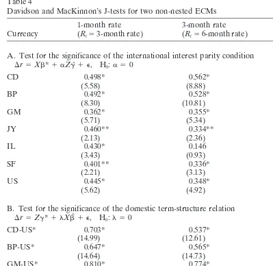
Table 4
Davidson and MacKinnon’s J-tests for two non-nested ECMs
1-month rate 3-month rate 6-month rate
Currency (Rt53-month rate) (Rt56-month rate) (Rt512-month rate)
A. Test for the significance of the international interest parity condition Dr5Xb*1 aZgˆ 1 e, H0:a 50
B. Test for the significance of the domestic term-structure relation Dr5Zg*1 lXbˆ 1 e, H0:l 50
* Indicates statistically significant differences from 0 at 1%. ** Indicates statistically significant differences from 0 at 5%. *** Indicates statistically significant differences from 0 at 10%. Numbers in parentheses aretstatistics.
Null hypothesis ofa 50 is used for testing significance of international interest rate parity condition. Null hypothesis ofl 50 is used for testing significance of domestic term-structure element.
behavior of short-term Eurocurrency rates. The results of the J-test are presented in
Table 4. For all cases of testingl 5 0, thetstatistics are highly significant, rejecting
the null. This suggests that the arguments involved in the term-structure relationship possess significant information to explain the changes of short rates. Similarly, the
test results support the argument that the international interest rate parity theory is valid for predicting short-rate movements, thus concurring the international integration hypothesis. Evidently, there is a complementary relationship between two-dimensional market arbitrage: intertemporal and international spatial.
On the basis of these findings, we re-estimate the short-term interest rate equations by combining the arguments in both the domestic term structure of interest rates and international interest rate parity ECMs. Two alternative approaches are considered for the model estimations. In the first approach, we combine the information involving
two-dimensional market cointegration. In this way, the error-correcting term, ut, is
obtained from Eq. (11), a regression equation:
rt5b01 b1Rt1b2r*ft 1ut. (11)
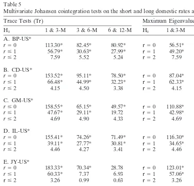
This equation assumes thatrtis cointegrated withRtandr*ft simultaneously. To verify
this presumption, we perform Johansen tests (1988, 1991) on the vector of [rtRtr*ft].
As shown in Table 5, both the trace test and the maximum eigenvalue test produce very similar results. The evidence shows that the hypothesis of no cointegrating vector is rejected. The only exception is the 6-month rate for the JY, where the null cannot be rejected. Next, we examine the hypothesis that the number of the cointegrating vectors is at most equal to 1. The null is also rejected. These test results thus suggest that, with the exception of the JY, there are two cointegrating vectors for the system. This means these three variables have a meaningful long-run relationship and do not tend to move too far away from each other. Having derived the error correcting term, we can write the ECM as follows:
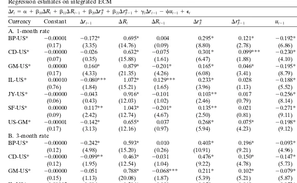
Drt5 a 1 b10DRt1 b11DRt211 b20Dr*ft 1 b21Dr*ft211 g1Drt21
2cut211 et (12)
In the second approach to combine term-structure and interest rate parity informa-tion, we include both error-correcting terms derived from the long-run equilibrium Eqs. (1) and (3), respectively, into the ECM specification. Specifically, we write
Drt5 a 1 b10DRt1 b11DRt211 b20Dr*ft 1 b21Dr*ft211 g1Drt21
2 c1u1,t212 c2u2,t211 et (13)
This specification allows us to detect the relative effect of two alternative adjustment processes. The estimates of Eqs. (12) and (13) are reported in Tables 6 and 7, respec-tively. The evidence shows that all of the estimated regressions have a relatively high
R2, ranging from 0.70 to 0.95. TheseR2s derived from the combined error-adjustment
effect are higher than those derived from either the domestic term-structure model or the interest rate parity condition. Several empirical findings are worth noting.
Table 5
Multivariate Johansen cointegration tests on the short and long domestic rates and effective foreign rate
Trace Tests (Tr) Maximum Eigenvalue Tests (lmax)
H0 1 & 3-M 3 & 6-M 6 & 12-M H0 1 & 3-M 3 & 6-M 6 & 12-M A. BP-US*
r50 113.30* 82.45* 80.92* r50 56.51* 51.82* 52.93*
r#1 56.79* 30.63* 27.99* r51 49.20* 25.12* 22.75*
r#2 7.59 5.52 5.24 r52 7.59 5.52 5.24
B. CD-US*
r50 153.52* 95.11* 78.50* r50 87.04* 50.12* 46.26*
r#1 66.48* 44.99* 32.23* r51 62.33* 40.49* 28.85*
r#2 4.15 4.50 3.38 r52 4.15 4.50 3.38
C. GM-US*
r#0 158.55* 65.15* 49.57* r50 110.88* 36.04* 29.85*
r#1 47.67* 29.11* 19.72 r51 42.98* 24.21* 15.39
r#2 4.69 4.90 4.33 r52 4.69 4.90 4.33
D. IL-US*
r50 155.41* 74.26* 71.49* r50 116.30* 46.49* 40.68*
r#1 39.11* 27.77* 30.81* r51 34.65* 23.50* 27.40*
r#2 4.46 4.27 3.41 r52 4.46 4.27 3.41
E. JY-US*
r50 183.33* 70.34* 28.78 r50 123.01* 62.97* 21.84
r#1 60.33* 7.37 6.93 r51 57.06* 6.39 6.31
r#2 3.26 0.99 0.63 r52 3.26 0.99 0.63
F. SF-US*
r50 228.13* 86.36* 102.67* r50 132.76* 51.95* 58.83*
r#1 95.36* 34.41* 43.84* r51 87.66* 27.42* 36.88*
r#2 7.70 6.99 6.96 r52 7.70 6.99 6.96
G. US-GM*
t50 174.66* 96.90* 94.35* r50 96.06* 62.79* 64.51*
r#1 78.60* 34.12* 29.84* r51 73.55* 28.92* 25.04*
r#2 5.05 5.20 4.80 r52 5.05 5.20 4.80
* indicates statistically significant at the 5% level. Trace (0.95) andlmax (0.95) are critical values for trace tests and maximum eigenvalue tests at the 95% quartile of the distribution. These critical values were taken from Osterwald-Lenum (1992).
Trace (0.95) lmax (0.95)
r50 34.91 r50 22.00
r#1 19.96 r51 15.67
r#2 9.24 r52 9.24
→
Kim
/
International
Review
of
Economics
and
Finance
9
(2000)
157–179
CD-US* 20.00000 20.026 0.632* 20.075 0.301* 0.099*** 20.230* 0.85 0.0011 2.08 (0.07) (0.35) (15.88) (1.61) (6.47) (1.88) (4.10)
GM-US* 0.00000 0.160* 0.879* 20.201* 0.165* 0.046* 20.195* 0.84 0.0009 1.96 (0.17) (4.33) (21.35) (4.26) (6.08) (3.41) (8.79)
IL-US* 0.00010 20.080*** 1.072* 0.129*** 0.233* 0.028 20.188* 0.89 0.0032 2.02 (0.76) (1.84) (15.21) (1.65) (3.96) (1.13) (5.52)
JY-US* 20.00000 20.043 0.916* 20.101 0.103** 0.017 20.256* 0.70 0.0014 1.75 (0.06) (0.43) (12.03) (1.02) (2.46) (0.79) (8.14)
SF-US* 0.00000 0.117** 1.043* 20.201* 0.135** 0.021 20.271* 0.77 0.0018 1.98 (0.09) (2.42) (12.74) (4.67) (2.50) (0.81) (9.11)
US-GM* 20.00001 20.142* 0.655* 0.037 0.268* 0.075* 20.198* 0.85 0.0012 2.00 (0.17) (3.13) (12.16) (0.97) (5.94) (4.23) (9.12)
B. 3-month rate
BP-US* 20.00000 20.242* 0.593* 0.010 0.403* 0.196* 20.093* 0.91 0.0010 2.11 (0.12) (4.98) (15.20) (0.26) (10.91) (9.21) (4.96)
CD-US* 20.00000 20.099** 0.463* 20.031 0.476* 0.150* 20.147* 0.91 0.0008 2.09 (0.12) (1.95) (12.54) (1.04) (9.22) (4.78) (5.73)
GM-US* 20.00000 20.051 0.788* 20.068*** 0.211* 0.102* 20.079* 0.88 0.0006 2.05 (0.15) (1.13) (20.08) (1.87) (5.39) (5.21) (5.87)
IL-US* 0.00005 20.004 1.204* 0.091 0.058 20.049 20.052* 0.80 0.0026 1.96 (0.60) (0.13) (6.28) (0.92) (0.82) (1.26) (2.68)
JY-US* 20.00000 20.029 0.855* 20.048 0.127** 0.060 20.076* 0.83 0.0009 2.00 (0.14) (0.51) (12.90) (0.78) (2.45) (1.51) (4.02)
SF-US* 0.00000 20.187* 0.851* 0.124* 0.213* 0.084* 20.108* 0.88 0.0009 2.04 (0.15) (4.48) (11.55) (3.51) (3.22) (3.01) (5.26)
US-GM* 20.00000 20.069 0.700* 20.026 0.272* 0.100* 20.107* 0.95 0.0007 2.04 (0.14) (1.23) (13.52) (0.77) (5.09) (3.10) (6.11)
→
/
International
Review
of
Economics
and
Finance
9
(2000)
157–179
173
Drt5 a 1 b10DRt1 b11DRt211 b20Dr*ft 1 b21Dr*ft211 g1Drt212 cut211 et
Currency Constant Drt21 DRt DRt21 Dr*ft Dr*ft21 ut21 R2 SEE DW
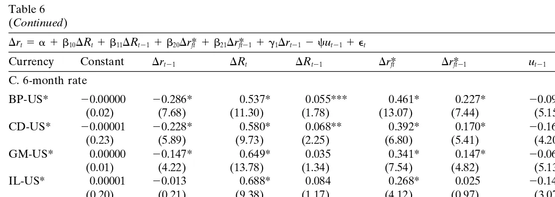
C. 6-month rate
BP-US* 20.00000 20.286* 0.537* 0.055*** 0.461* 0.227* 20.091* 0.92 0.0009 2.12 (0.02) (7.68) (11.30) (1.78) (13.07) (7.44) (5.15)
CD-US* 20.00001 20.228* 0.580* 0.068** 0.392* 0.170* 20.162* 0.91 0.0008 2.11 (0.23) (5.89) (9.73) (2.25) (6.80) (5.41) (4.20)
GM-US* 0.00000 20.147* 0.649* 0.035 0.341* 0.147* 20.066* 0.89 0.0005 2.09 (0.01) (4.22) (13.78) (1.34) (7.54) (4.82) (5.13)
IL-US* 0.00001 20.013 0.688* 0.084 0.268* 0.025 20.147* 0.78 0.0019 1.97 (0.20) (0.21) (9.38) (1.17) (4.12) (0.97) (3.07)
JY-US* 20.00000 20.012 0.919* 20.031 0.137** 0.040 20.067* 0.80 0.0008 1.98 (0.06) (0.19) (14.06) (0.54) (2.27) (0.94) (3.81)
SF-US* 20.00000 20.100** 0.846* 0.049 0.203* 0.077* 20.090* 0.86 0.0008 2.02 (0.02) (2.36) (16.20) (1.14) (4.11) (3.04) (5.70)
US-GM* 20.00000 20.149* 0.564* 20.024 0.464* 0.152* 20.136* 0.95 0.0006 2.07 (0.16) (2.79) (9.18) (0.59) (9.23) (4.12) (5.38)
→
Kim
/
International
Review
of
Economics
and
Finance
9
(2000)
157–179
BP-US* 20.00001 20.173* 0.695* 0.005 0.295* 0.123* 20.108* 20.081* 0.86 0.0016 2.37 (0.17) (3.39) (14.51) (0.11) (8.52) (2.87) (5.25) (4.56)
GM-US* 0.00000 0.160* 0.880* 20.204* 0.162* 0.049* 20.150* 20.041* 0.84 0.0009 1.96 (0.17) (4.30) (21.04) (4.29) (5.71) (3.92) (8.75) (3.93)
IL-US* 0.00010 20.077*** 1.087* 0.121 0.221* 0.038 20.192* 20.002* 0.89 0.0032 2.02 (0.81) (1.76) (13.70) (1.54) (3.48) (1.63) (6.43) (0.16)
JY-US* 20.00000 20.048 0.914* 20.088 0.105** 0.016 20.165* 20.082* 0.70 0.0014 1.75 (0.06) (0.48) (11.56) (0.87) (2.27) (0.87) (7.24) (4.37)
SF-US* 0.00000 0.114** 1.042* 20.199* 0.133** 0.023 20.181* 20.083* 0.77 0.0018 1.98 (0.09) (2.30) (12.31) (4.38) (2.29) (1.03) (7.57) (4.25)
US-GM* 20.00001 20.144* 0.651* 0.042 0.272* 0.072* 20.089* 20.109* 0.85 0.0012 2.00 (0.18) (3.19) (11.08) (1.06) (5.55) (4.36) (4.85) (5.07)
B. 3-month rate
BP-US* 20.00000 20.242* 0.597* 0.007 0.399* 0.198* 20.046* 20.045* 0.91 0.0010 2.11 (0.12) (4.91) (14.85) (0.18) (10.43) (9.46) (4.54) (2.99)
CD-US* 20.00000 20.102** 0.470* 20.039 0.466* 0.159* 20.066* 20.077* 0.91 0.0008 2.10 (0.13) (2.01) (12.66) (1.36) (9.08) (4.77) (6.20) (3.97)
GM-US* 20.00000 20.051 0.790* 20.071*** 0.209* 0.104* 20.054* 20.024* 0.88 0.0006 2.05 (0.15) (1.13) (20.03) (1.95) (5.27) (5.47) (5.44) (3.47)
IL-US* 0.00005 20.004 1.197* 0.093 0.062 20.053 20.049** 20.003 0.81 0.0026 1.95 (0.58) (0.12) (6.23) (0.93) (0.89) (1.28) (2.32) (0.26)
JY-US* 20.00000 20.030 0.855* 20.050 0.126*** 0.064*** 20.067* 0.006 0.83 0.0009 2.00 (0.16) (0.53) (12.86) (0.82) (2.40) (1.71) (3.90) (1.13)
SF-US* 0.00000 20.187* 0.851* 0.124* 0.213* 0.084* 20.060* 20.048* 0.88 0.0009 2.04 (0.15) (4.48) (11.47) (3.50) (3.19) (3.08) (4.29) (4.87)
US-GM* 20.0000 20.069 0.701* 20.027 0.271* 0.101* 20.027** 20.079* 0.95 0.0007 2.04 (0.14) (1.21) (13.17) (0.77) (4.95) (3.16) (2.50) (4.35)
→
/
International
Review
of
Economics
and
Finance
9
(2000)
157–179
175
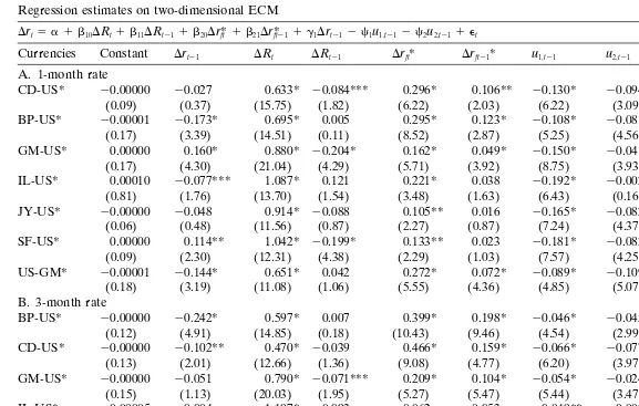
Drt5 a 1 b10DRt1 b11DRt211 b20Dr*ft 1 b21Drft*211 g1Drt212 c1u1,t212 c2u2,t211 et
Currencies Constant Drt21 DRt DRt21 Drft* Drft21* u1,t21 u2,t21 R2 SEE DW
C. 6-month rate
BP-US* 20.00000 20.287* 0.538* 0.055*** 0.460* 0.228* 20.027* 20.063* 0.92 0.0009 2.12 (0.02) (7.72) (11.05) (1.81) (12.76) (7.59) (3.35) (3.93)
CD-US* 20.00001 20.229* 0.584* 0.065** 0.387* 0.175* 20.052* 20.107* 0.91 0.0008 2.11 (0.23) (5.91) (9.68) (2.05) (6.63) (5.55) (4.33) (3.38)
GM-US* 0.00000 20.147* 0.649* 0.034 0.340* 0.148* 20.025* 20.040* 0.89 0.0005 2.09 (0.01) (4.22) (13.64) (1.30) (7.43) (4.90) (4.36) (4.06)
IL-US* 0.00001 20.014 0.668* 0.086 0.267* 0.026 20.090* 20.054** 0.78 0.0019 1.97 (0.20) (0.23) (9.15) (1.19) (4.11) (1.05) (3.63) (2.36)
JY-US* 20.00000 20.014 0.919* 20.033 0.136** 0.045 20.062* 20.003 0.80 0.0008 1.98 (0.08) (0.22) (14.13) (0.55) (2.24) (1.12) (3.54) (0.63)
SF-US* 20.00000 20.100** 0.851* 0.045 0.198* 0.082* 20.050* 20.037* 0.86 0.0008 2.03 (0.02) (2.36) (16.08) (1.03) (3.99) (3.23) (4.28) (2.79)
US-GM* 20.00000 20.149* 0.563* 20.023 0.465* 0.151* 20.009 20.128* 0.95 0.0006 2.07 (0.16) (2.79) (9.02) (0.56) (9.10) (4.14) (1.31) (5.01)
the coefficients foru1,t21in general are higher than those ofu2,t21, indicating that the
domestic term-structure force carries more weight in the adjustment process.
It is important to point out that the estimated coefficients of the error-correcting
terms from Eq. (12),c, are approximately equal to the sum of the values of two
error-correcting terms,c11 c2, based on Eq. (13). This suggests that the information of
the combined error-correcting term, ut21, summarizes the effects that come from
domestic,u1,t21, and international,u2,t21, adjustment processes.
Second, all the contemporaneous terms of the change in the long rates and the change of the effective foreign short rates (Eurodollar rates plus forward premium on U.S. dollar) shown in both Tables 6 and 7 have a positive sign and are highly statistically significant. In addition, the one-period lagged rates are also significant in about half the cases, although they are much weaker. In terms of magnitude, the current change in long rates is, in general, larger than that of effective foreign short rates. Thus, the evidence favors the elements involved in utilizing the domestic term structure of interest rates to describe the short-rate movements.
6. Conclusion
This paper investigates short-term interest rate behavior, applying the data from seven Eurocurrency rates. Unit-root tests suggest that both levels of short-end Eurocur-rency deposit rates and effective foreign interest rates (Eurodollar deposit rates plus forward premiums) are nonstationary. We find evidence for two-dimensional cointe-gration: the domestic short rate cointegrated with the long rate of the same currency and the domestic short rate cointegrated with the effective foreign short rate having the same maturity.
By building on established evidence that the short-term interest rate is more appro-priate for specification in an error-correction model based on the domestic term-structure relationship (Chiang & Chiang, 1995), this paper adds a new element to the model: the international interest rate parity ECM. Our empirical evidence indicates that both error-correcting terms, derived from the domestic term-structure relationship and the interest rate parity condition, are highly significant. Thus, these two error-correcting terms can be used simultaneously to predict subsequent short-rate move-ments. Yet, when the estimations are based on the combined error-correcting term, by regressing the domestic short rate on both the domestic long rate and the effective foreign short rate, the estimated value of this coefficient in the ECM is approximately equal to the sum of two individual error-correcting terms, producing a combined effect in predicting short rates.
This finding has an important policy implication, because our evidence indicates that market adjustments react not only to the deviations of the current short rate from its long-run level, but also to the divergences of international interest rates. To make monetary policy effective and at the same time maintain a stable financial market system, a closer coordination between international monetary authorities is necessary.
foreign short rate are highly significant in explaining short-term interest rate behavior. We conclude that both arguments shown in the domestic term structure of interest rates as well as the international interest rate parity equation are relevant for predicting short-term interest rates. Although these two market arbitrages are complementary, the domestic term-structure elements appear to have more significant explanatory power than does the international dimension.
Notes
1. The sample period spans June 1, 1973, to August 2, 1996. This period applies to the data for the U.S. dollar, GM, and SF. However, with the same ending period, the starting periods for the data series vary across the other currencies and maturities. For the case of BP, the starting period is June 1, 1973, for the 1-, 3-, and 6-month rates and September 21, 1973, for the 12-month rate. In the case of CD, the sample period starts from August 17, 1979, for 1-, 3-, and 6-month rates and September 21, 1973, for the 12-month rate. In the case of JY, the sample period starts from January 6, 1978, for the 3-, 6-, and 12-month rates and January 5, 1979, for the 1-month rate. For the IL, all the data start from October 3, 1980. For the foreign exchange rates, with the exceptions of 12-month forward exchange rates for JY and IL, all sample periods start from June 1, 1973. The data for the 12-month forward exchange rate starts from December 28, 1973, for IL and January 18, 1974, for JY. French franc rates were excluded from our study because their failure to satisfy the necessary condition of the cointegration tests.
2. Similar results were obtained from the Phillips and Perron test (1998).
3. Johansen (1988, 1991) and Johansen and Juselius (1990) provide an alternative approach for investigating cointegration relations on the multivariate approach. According to Johansen’s approach, the cointegrating vectors are determined by the ranks in the cointegrating matrix, suggesting two likelihood-ratio statistics to determine the number of cointegrating vectors. These two statistics are trace statistics and maximum eigenvalue statistics. The trace statistic is defined as:
22ln(Q) 5 2T Sp
i5r11ln(1 2 lˆi), where lˆr11, . . . , lˆp are the p 2 r smallest
eigenvalues. The trace statistic tests the null hypothesis that the number of
distinct cointegrating vectors is less than or equal toragainst a general
alterna-tive. Next, the maximum eigenvalue statistic is given by22ln(Q)5 2Tln(12
lr11). The null hypothesis tested by the maximum eigenvalue statistic is that the
number of cointegrating vectors isragainst the alternative,r11 cointegrating
international adjustment is more sensitive and effective for the short-end hori-zons. To save space, the Johansen test results are not reported here.
4. To achieve a consistent estimator, the White (1980) and Newey and West (1985) procedure has been used to obtain the estimates in Tables 2, 3, and 5. The White-Newey-West estimate of the variance–covariance matrix allowing for
conditional heteroskedasticity is given byVˆ(bˆ )5(X9X)21Wˆ(X9X)21, whereX
denotes the right-hand side variables. The matrix Wˆ is calculated by
Wˆ 5
o
Whenuis equal to 0, the weight becomes unity andWˆ reduces to Hansen and
Hodrick’s specification (1980). A special case occurs whenu 51, which is the
smallest value that guarantees a positive definite matrix (Doan, 1991).
5. Our testing results (not reported) indicate that both [b10b11]9 5[0 1]9and [b20
b21]9 5 [0 1]9 are rejected in most cases. This evidence means thatu1,tand u2,t
are not necessarily equal to (rt2Rt) and (rt2r*ft), respectively. However,u1,t
andu2,tdo summarize some information about return spreads, imperfect
substi-tutability, and different preferences toward different instruments. From the
econometric point of view, the error-correcting terms, such asu1,tandu2,t, possess
useful informational content for predicting future interest rate movements. 6. Note that the magnitudes of the coefficients of the error-correction terms in this study are consistently smaller than those of Chiang and Chiang (1995). This result comes from the use of a different frequency of the data. Chiang and Chiang (1995) use monthly data, while we use weekly data; thus, the coefficients of the error-correction terms represent a weekly adjustment rather than a monthly adjustment.
References
Abeysekera, S. P., & Turtle, H. J. (1995). Long-run relations in exchange markets: a test of covered interest parity.Journal of Financial Research 18, 431–447.
Arshanapalli, B., & Doukas, J. (1994). Common stochastic trends in a system of Eurocurrency rates. Journal of Banking and Finance 18, 1047–1061.
Atkins, F. J. (1993). The dynamics of adjustment in deviations from covered interest parity in the Euromarket: evidence from matched daily data.Applied Financial Economics 3, 183–187.
Bhatti, R. H., & Moosa, I. A. (1995). An alternative approach to testing uncovered interest parity. Applied Economic Letters 2, 478–481.
Boothe, P. (1991). Interest parity, cointegration, and the term structure in Canada and the United States. Canadian Journal of Economics 24, 595–603.
Bradley, M. G., & Lumpkin, S. A. (1992). The treasury yield curve as a cointegrated system.Journal of Financial and Quantitative Analysis 27, 449–463.
Chiang, T. C., & Chiang, J. J. (1995). Empirical analysis of short-term Eurocurrency rates: Evidence from a transfer function error correction model.Journal of Economics and Business 47, 335–351. Choi, S., & Wohar, M. E. (1991). New evidence concerning the expectations theory for the short end
of the maturity spectrum.Journal of Financial Research 14, 83–92.
Committeri, M., Rossi, S., & Santorelli, A. (1993). Tests of covered interest parity on the Euromarket with high-quality data.Applied Financial Economics 31, 89–93.
Davidson, R., & MacKinnon, J. (1981). Several tests for model specification in the presence of alternative hypotheses.Econometrica 49, 781–793.
Dickey, D. A., & Fuller, W. A. (1979). Distribution of the estimators for autoregressive time series with a unit root.Journal of the American Statistical Association 74, 427–431.
Dickey, D. A., & Fuller, W. A. (1981). Likelihood ratio statistics for autoregressive time series with a unit root.Econometrica 49, 1057–1072.
Doan, T. A. (1991).RATS Users’ Manual.Evanston, IL: Estima.
Engle, R. F., & Granger, C. W. J. (1987). Co-integration and error correction: representation, estimation, and testing.Econometrica 55, 251–276.
Engsted, T., & Tanggaard, C. (1994). Cointegration and the US term structure.Journal of Banking and Finance 18, 167–181.
Fuller, W. A. (1976).An Introduction to Statistical Time Series.New York: Wiley.
Hall, A. D., Anderson, H. M., & Granger, C. W. J. (1992). A cointegration analysis of Treasury bill yields.Review of Economics and Statistics 74, 116–126.
Hansen, L. P., & Hodrick, R. J. (1980). Forward exchange rates as optimal predictor of future spot rates: an econometric analysis.Journal of Political Economy 88, 829–853.
Johansen, S. (1988). Statistical analysis of cointegration vectors.Journal of Economic Dynamics and Control 12, 231–254.
Johansen, S. (1991). Estimation and hypothesis testing of cointegration vectors in Gaussian vector autoregressive models.Econometrica 59, 1551–1580.
Johansen, S., & Juselius, K. (1990). Maximum likelihood estimation and inference on cointegration-with applications to the demand for money.Oxford Bulletin of Economics and Statistics 52, 169–210. Kugler, P. (1990). An empirical note on the term structure and interest rate stabilization policies.Journal
of International Money and Finance 9, 234–244.
Mehra, Y. P. (1993). The stability of the M2 demand function: evidence from an error correction model. Journal of Money, Credit and Banking 25, 455–460.
Modigliani, F., & Sutch, R. (1966). Innovations in interest rate policy.American Economic Review 56, 178–197.
Mougoue, M. (1992). The term structure of interest rates as a cointegrated system: Empirical evidence from the Eurocurrency market.Journal of Financial Research 15, 285–296.
Muscatelli, V. A., & Jurn, S. (1992). Cointegration and dynamic time series models.Journal of Economic Survey 6, 1–43.
Newey, W. K., & West, K. D. (1987). A simple, positive semi-definite, heteroskedasticity and autocorrela-tion consistent covariance matrix.Econometrica 55, 703–708.
Nourzad, F., & Grennier, R. S. (1995). Cointegration analysis of the expectations theory of the term structure.Journal of Economics and Business 47, 281–292.
Osterwald-Lenum, M. (1992). A note with quantiles of the asymptotic distribution of the maximum likelihood cointegration rank test statistics.Oxford Bulletin of Economics and Statistics 54, 461–472. Phillips, P. C. B., & Perron, P. (1988). Testing for a unit root in time series regression.Biometrika 75,
335–346.
West, K. D. (1988). Asymptotic normality, when regressors have a unit root.Econometrica 56, 1397–1417. White, H. (1980). A heteroskedasticity-consistent covariance matrix estimator and a direct test for