An approach to deriving roughness length and zero-plane displacement
height from satellite data, prototyped with BOREAS data
K.J. Schaudt
a,∗, R.E. Dickinson
b,1aUniversity of Arizona, Institute of Atmospheric Physics, Tucson, AZ 85721, USA
bGeorgia Institute of Technology, Earth and Atmospheric Sciences, 221 Bobby Dodd Way, Atlanta, GA 30332-0340, USA Received 19 August 1999; received in revised form 3 April 2000; accepted 5 April 2000
Abstract
Global climate models typically use relatively crude estimates of roughness length, often based on constant values for land cover category. However, large variations may exist within any of the vegetation categories. Global large-scale estimates of roughness length, such as required by climate models, cannot rely on field experiments for practical reasons and must, therefore, be derived from satellite observations. This paper develops a satellite retrieval method for the roughness parameters, momentum roughness length, zo, and displacement height, d. The formulas, based on the observational data of Raupach
[Raupach, M.R., 1992. Bound.-Layer Meteor. 60, 375–395; Raupach, M.R., 1994. Bound.-Layer Meteor. 71, 211–216] and Lindroth [Lindroth, A., 1993. Bound.-Layer Meteor. 66, 265–272], are applicable to most types of vegetation. Raupach relates the momentum roughness length and zero-plane displacement height to the frontal area index,λ, and to the height of the vegetation, h. The frontal area index is related to the shape of an average tree or plant crown and to the average density of the canopy elements. The crown shape factor includes the aspect (height-to-width) ratio of the crown and the geometric shape of the crown. Lindroth relates the momentum roughness length to the leaf area index (LAI) and to the height of the trees.
The functional form of zo/h is peaked in both frontal area index, with the maximum occurring atλ=0.152, and average
plant LAI (Lp), with the maximum occurring at Lp=0.878. Asλand Lpincrease, d/h also increases and approaches an upper
limit asymptotically at high values ofλand Lp.
As the vegetation height is difficult to obtain from present satellite data, retrievals are restricted to fractional values (i.e.
zo/h and d/h) for global application. This retrieval then requires data for the crown aspect ratio, the canopy density (fractional
overstory canopy cover) and the LAI. Data from BOREAS (BOReal Ecosystem Atmosphere Study) are used to illustrate this satellite retrieval method. © 2000 Elsevier Science B.V. All rights reserved.
Keywords: Aerodynamic roughness; Remote sensing; Frontal area index; Leaf area index
1. Introduction
Aerodynamic roughness length, a significant factor in climate models, depends on the height and spacing
∗Corresponding author. Tel.:+1-520-621-6015; fax:+1-520-621-6833.
E-mail addresses: [email protected] (K.J. Schaudt),
[email protected] (R.E. Dickinson) 1Tel.:
+1-404-385-1509; fax:+1-404-894-5638.
of the largest objects acting to retard the surface air-flow. For vegetated areas these objects are the canopy elements. Roughness length has commonly been es-timated for local sites from vertical wind profiles and micrometeorological theory. However, scaling to areas of individual climate model grid cells require estimates from satellite remote sensing. In the absence of such estimates, climate modelers have used a land cover characterization with a roughness length
ciated with each land-cover type. This association has commonly been done by assigning a physical height to the canopy of each land-cover type and a pre-scribed ratio of roughness length-to-physical height of the given canopy. Although it would appear that any real large-scale measurement should be able to improve this crude approach, development of satellite approaches have only recently begun to provide such a measurement. Jasinski and Crago (1999) developed a method of estimating the aerodynamic roughness of vegetated surfaces. The research presented in this paper differs in general approach from that of Jasinski and Crago. The formulas developed here also directly include the effects of leaf area index (LAI), which they do not consider.
Separating the effects of LAI from the effects of plant spacing and shape has additional advantages for modelers. Many land-cover types (e.g. forests, shrub-land, semi-desert and savannas) have major canopy elements that change shape but little within a sin-gle growing season, whereas the LAI may have large changes over the growing season as a result of decid-uous behavior, herbivory or harvest. These changes in LAI can either be prescribed from remote sensing (see, e.g. Sellers et al., 1996) or modeled interactively as a part of the climate system (see, e.g. Dickinson et al., 1998).
Micrometeorologists have long recognized (see, Garratt, 1994) that the ratio of roughness length zoto
canopy height h widely varies. This ratio would be expected to decrease as a canopy fills in and the air flow experiences drag only near the top of the canopy. Conversely, as canopy elements become sparse, the drag they exert, and hence this ratio, should again de-cline. Therefore, this ratio should maximize at some intermediate value of canopy density. The canopy pa-rameter that determines this dependence is the crown frontal (horizontal) area multiplied by the canopy element density. The crown frontal area depends on the crown aspect (height-to-width) ratio (CAR) and the geometric shape of the crown. Raupach (1992, 1994) provides a good observational basis for relat-ing zo/h to the product of the crown frontal area and
a density parameter. This product is given the name ‘frontal area index’. His observations were largely performed on densely vegetated or solid objects, and therefore do not indicate what corrections might be expected when leaf area is sparse. Lindroth (1993)
supplies such corrections for the LAI. The zo/h ratio
should decrease with increasing density in foliage as the drag would be exerted by only the outermost leaves and branches. This ratio may again decrease for sparse-enough canopies, such as bare branches, because of the reduction in the resistance to the air flow. Again, at some intermediate level of LAI, there should be a maximum value for zo/h. Numerical
stud-ies by Seginer (1974), Kondo and Akashi (1976) and Shaw and Pereira (1982) also predict this behavior.
Surface roughness over a large area could, there-fore, be supplied from satellite data that provides the following variables: (i) canopy height; (ii) canopy den-sity; (iii) crown aspect ratio; and (iv) LAI. Estimates of the fractional vegetation cover and the LAI can now be obtained from existing NOAA AVHRR radi-ance archives (see Eidenshink and Faundeen, 1994). The average CAR can be roughly estimated based on field observations. However, the height of the canopy may be best estimated from a canopy lidar, such as the planned vegetation canopy lidar (VCL). Hence, prior to the availability of this data we limit retrievals to fractional values (zo/h and d/h).
Latent and sensible heat fluxes have the greatest sensitivity to the roughness length for the tallest veg-etation as demonstrated by Pitman (1994). Further-more, the neutral drag coefficient is proportional to the square of the natural logarithm of the roughness length. Consequently, at 10 m above the surface, a 10% change in zoat zo=0.01 produces a 2.8% change
in the neutral drag coefficient, but an 8.5% change for zo=1.0. At small roughness length, appropriate to
short vegetation, the ratio of sensible-to-latent heat fluxes (the Bowen ratio) is largely energy controlled and, therefore, relatively insensitive to zo, although the
difference between skin temperature and air tempera-ture depends on zo. Conversely, at large zo, appropriate
to tall vegetation, the partitioning of energy between latent and sensible heats, as needed in climate mod-els, is relatively sensitive to percent errors in zo, but
departures of skin temperature from air temperature are less sensitive as compared to short vegetation (see Dickinson, 1983, for a more complete discussion).
and evergreen) is also surveyed. Section 3 illustrates the application of the formulas to a portion of the BOREAS Southern Study Area (SSA). The BOREAS archives include data on the average canopy height, fractional canopy cover and LAI. Satellite retrievals over this same area are also given. Section 4 discusses likely limitations and inaccuracies incurred by use of currently available satellite data. The near-future improvements in the satellite derived roughness pa-rameters, which arise from new or improved satellite observations, are also discussed. Section 5 summa-rizes the paper.
2. Formulas and Methodology
The parameterization of roughness length and displacement height is based on two sources. The dependence of the roughness length, zo, and the
displacement height, d, on the frontal area index is inferred from Raupach (1992, 1994). The depen-dence of d and zo on LAI is from Lindroth (1993).
Although the iterative method, which was used to obtain the roughness parameters in Raupach’s work, has recently been proven to often produce inaccurate roughness parameters (see, Schaudt, 1998), his results are still reasonable and will be used as is, because the data is not available for reanalysis. The iterative method’s roughness parameter retrievals is likely to have an error of no more than 10–15%, with the sign of individual errors difficult to predict. The errors in
zoand d are roughly equal in magnitude and typically
opposite in sign.
Raupach related the frontal area index, denoted by λ, to the roughness length and displacement height. The parameter λ is defined as the frontal area (area from a horizontal point of view, denoted by Af) per
unit ground area. The frontal areas, Af, for trees (more
generally, elliptic and conic plants) are for broad-leaf trees
where hs and ws, respectively, are the height of the
stem to the base of the crown and the average width
of the stem (between the ground and the base of the crown) and hcand wc, respectively, are the height and
width of the crown of the tree or plant. The frontal area index can then be found by multiplying Af by the
number of plants per unit ground area (which is equiv-alent to dividing Af by the average distance between
the plants squared). The average distance between the plants can be related to the fractional canopy cover,
fc, and the width of the crown wc as
The average distance described in Eq. (3) is only pre-cisely valid for uniformly spaced trees. For randomly spaced trees, the mean distance to the nearest neighbor is the appropriate measure to use. However, the differ-ence between the two conditions will not be consid-ered here. The fractional canopy cover is that fraction of the area (as viewed from above) which is covered by the overstory canopy. For areas with significant un-derstory growth, the fractional canopy cover and the fractional vegetation cover can vary significantly. Be-fore data from the VCL satellite is available, care will have to be taken for retrievals over certain land covers, such as savannas.
Assuming that the frontal area of the stem is much smaller than the frontal area of the crown, the frontal area indexes (λ=Af/D2) are approximated by λ=fc
hc wc
(4)
for broad-leaf trees (or elliptical plants) and
λ= 2 πfc
hc wc
(5)
for needle-leaf trees (or conical plants).
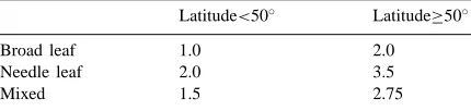
Table 1
The constant values of the crown aspect ratio for the initial rough-ness parameter product
Latitude<50◦ Latitude≥50◦
Broad leaf 1.0 2.0
Needle leaf 2.0 3.5
Mixed 1.5 2.75
by constant values for different vegetation types and locations as shown in Table 1. The average ratio of stem area-to-crown area was also determined from these data, and found to be less for broad-leaf trees than for needle-leaf trees, typically<5% of the crown area for both mid-latitude and boreal broad-leaf trees, for mid-latitude needle-leaf trees — <10% of the crown area and for boreal needle-leaf trees — averag-ing 25%, with a median value of<15%. For the boreal needle-leaf trees, a small number of trees with very small crowns biased the average high. Roughly 42% of the 723 boreal needle-leaf trees had stem frontal areas of<10% of the crown area and 72% had stem areas<20% of the crown area. Some species, such as palm trees, have crown aspect ratios consistently<1.0 (personal observations) and high stem-to-crown area ratios, but these types of trees usually do not cover vast areas. Errors in the estimation of zofrom ignoring
the stem area in the boreal needle-leaf trees will vary depending on the actual value ofλ. They are roughly 10–15% at the most sensitive values ofλ(roughly for
fc<0.15) and can be<2% for the least sensitive values
ofλ(for fc>0.3).
Figure 1c of Raupach (1994) illustrates the form of the dependence of zo/h on his canopy area index,
equal to twice the frontal area index for trees with isotropically oriented leaves. The value of zo/h peaks
atλ=0.152. Roughness length is related to the frontal area index, which is divided into two functions as fol-lows. Forλ=0.152 this can be expressed as
zo
value for bare soil. Eq. (6a) describes the upward leg of the zo/h function, and forλ>0.152 as
Fig. 1. The zo/h as a function of fractional canopy cover for various crown aspect ratios (CARs) for broad-leaf and needle-leaf forests. The axis are dimensionless for Figs. 1–4.
where a2=0.0537, b2=10.9, c2=0.874, d2=0.510 and
f2=0.00368. Eq. (6b) describes the downward leg of
the zo/h function. For vegetation of a normal shape,
ei-ther elliptical or conical, the value ofλrarely surpasses 5 so that the f2in Eq. (6b) is usually relatively small.
Raupach gives a more complex expression for zo/h.
Fig. 1 illustrates zo/h as a function of fractional canopy
cover for various values of crown aspect ratios (CARs) for both broad-leaf and needle-leaf trees. As this fig-ure illustrates, the fractional canopy cover at which
zo/h is maximum decreases and the peak narrows as
the crown ratio increases. Thereby, fully forested land (fc=1.0) with trees that have a high crown ratio have
a lower zo/h as compared to fully forested areas with
trees having a low crown ratio (Fig. 1).
The dependence of d/h on the frontal area index is given by Eq. (8) of Raupach (1994) as follows:
d
where a3=15.0. Fig. 2 illustrates d/h as a function
of fractional canopy cover for various CARs for broad-leaf and needle-leaf trees. As the crown ratio increases, the value for d/h at any given canopy cover also increases.
Observations of a willow forest by Lindroth are used to determine the dependence of d and zoon leaf area
index (LAI). Lindroth used three methods to retrieve
zoand d. Two of the methods are constant-d methods,
with two different ways of determining the value of
d, neither of which is proper (see Thom, 1975, for
Fig. 2. The d/h as a function of fractional canopy cover for various crown aspect ratios (CARs) for broad-leaf and needle-leaf forests.
third method used is that of Shaw and Pereira (1982), which is based on closure theory and is deemed more reasonable.
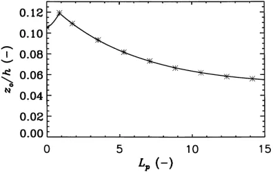
Lindroth, in his Fig. 5, illustrates the values of zo/h
as a function of LAI for the three different methods used. The open triangles represent the results from Shaw and Pereira’s method. In order to remove the influence of tree density on LAI which, in turn, will effect the roughness length, an average plant LAI,
Lp, was found. The LAI used by Lindroth is defined
as the average LAI per tree multiplied by the den-sity of trees (the tree denden-sity in the willow forest was 1.77 trees per square meter, from personal communi-cations with Lindroth). This can simply be inverted to give Lp. Satellite-derived LAI is typically given
as the total scene LAI. The Lp from the satellite is
then:
Lp= fv fc
LAI−fb fc
Lb (8)
where Lb is the LAI of the background and fb the
fraction of the area covered by only the understory vegetation (i.e. fv=fc+fb). The background LAI will
only be significant where a fairly large amount of understory vegetation exists and is easily visible to the satellites, such as in savannas and in some of the boreal forest. Ideally, the Lp should be used in
the following equations. Otherwise, with the use of the LAI, there is an undesirable mixing of Lp and fc
that will produce incorrect results. However, at high values of LAI, the difference in retrievals using LAI rather than Lpis relatively small, because the function
is relatively flat at high values of Lp.
Eqs. (6a) and (6b) are assumed to apply for infinite
Lp corresponding to either fully vegetated plants or
solid objects. Refinements would be possible if more information (i.e. the Lp of the vegetation in Fig. 1c
of Raupach) was available, but for his solid objects, the use of an infinite value for Lp in the
normaliza-tion is plausible. The equanormaliza-tions, which are found from Lindroth’s open triangles, are hence normalized to unity for infinite Lpproducing the following functions
for dependence of the roughness length:
fz=0.3299L1p.5+2.1713 for Lp<0.8775 (9a)
and
fc=1.6771 exp(−0.1717Lp)+1.0
for Lp≥0.8775 (9b)
The fit is shown in Fig. 3. This function, fz, then
is multiplied to the RHS of Eq. (6a) or Eq. (6b) to give roughness length as a function of both LAI and frontal area index. The limited number of points at low LAI makes the power of Lp in Eq. (9a)
some-what uncertain. The dependence of zo on Lp shows
a similar structure to that of frontal area index. That is, for the lowest and highest values of Lp, the
rough-ness length drops and there is a peak at some interme-diate value. Although the data of Lindroth is sparse in the peak area, the typical amount of time a tree spends in this range is relatively short (e.g. the wil-low trees studied by Lindroth had an Lpbetween zero
and 0.885 for only about 2 weeks in the spring and the fall). Hence, this uncertainty is only a factor dur-ing the sprdur-ingtime green-up and the autumn leaf-drop,
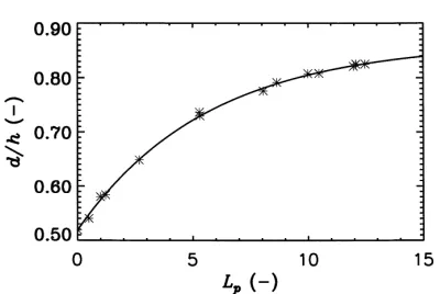
Fig. 4. The d/h vs. average plant LAI (Lp) developed from Fig. 1 of Lindroth (1993). As Lindroth’s figure did not include data points, rather only a line, the data points shown correspond to points on the lines taken at the same point in time. Data shown was analyzed with the method of Shaw and Pereira (1982).
and that too only for deciduous trees. The relatively short green-up and ledrop periods of time will af-fect only the monthly average in the months that they occur.
The dependence of d/h on Lp is developed from
Fig. 1 of Lindroth, which illustrates the value of d for the exact solution along with the mean height of the trees and the (average) LAI. Lindroth’s figure shows that d changes roughly 50% from bare trees to fully vegetated trees. Although there was some scatter in the values for d/h as a function of Lp, a reasonable fit
was still found, see Fig. 4. The displacement height d in Eq. (7) is multiplied by the following factor, again normalized for infinite Lp:
fd=1.0−0.3991 exp(−0.1779Lp) (10)
In the willow forest studied by Lindroth, the frac-tional canopy cover remained close to 100% through-out the entire season (Lindroth, personal communi-cations), so effects of changing fc are minimal. As
there may have been some unknown changes (likely increases) in CAR over the single season of Lindroth’s observations, it is possible that Eqs. (9a), (9b) and (10) slightly overestimate the effects of changing LAI. However, the maximum possible increase in the CAR is 50% (obtained from the change in height and the that fact fcstayed near 1.0). This change accounts for <1/10 of the observed changes in zo/h and<1/20 of
the observed change in d/h.
Obtaining the roughness parameter ratios (zo/h and
d/h), requires fractional canopy cover (fc), crown
as-pect ratio (hc/wc), and average plant LAI (Lp). Section
3 discusses how these variables will be estimated from satellite data. The retrieval is illustrated with observa-tions from a portion of the BOREAS SSA.
3. Satellite retrieval
The fractional vegetation cover of Zeng et al. (2000) is used because of its formulation for use with cli-mate models. We also assume a pixel average LAI is available independent of the fractional vegetation cover. This assumption may be problematical if LAI products are used that have assumed in their deriva-tion a given value for fracderiva-tional vegetaderiva-tion. In this case, the LAI is modified by multiplying by (fa/fv),
where fa is the assumed value of fractional vegetation
cover used in the satellite retrieval. Land covers with considerable understory vegetation, such as savannas and semi-deserts, require more care, as discussed in Section 4. Although typically large amounts of under-growth are present in boreal forests (including mature ones), analysis of the data from the BOREAS SSA indicates smaller errors than might have been antici-pated.
As vegetation height is available for the portion of the BOREAS area used here, the values of zo and d
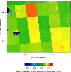
are retrieved, rather than their fractional values. Fig. 5 illustrates the results from the retrieval for a roughly 34 km by 43 km area within the BOREAS Southern Study Area (SSA) field program. This data is a com-bination of satellite, aircraft and ground truth obser-vations for land-cover type, LAI, fractional canopy cover and vegetation height at a resolution of 30 m (see Chen and Geng, 2000 and Gruszka, 1998 for details of these high quality observations). Retrievals used the CAR given in Table 1. The large area near the upper right-hand corner, with relatively low rough-ness length, corresponds to an area of relatively recent burn. Two lakes are visible in the image, both on the left side, and considerable other heterogeneity is seen here.
Fig. 5. The retrieved roughness length (in m) for 30-m BOREAS data for fc, Lp, h and land cover type, with the crown ratio given in Table 1.
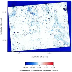
obtained from AVHRR satellites, by the method of DeFries et al. (1997) and with care may be able to produce the desired fractional canopy cover. However, we use the fractional vegetation cover (see Zeng et al., 2000) for the retrievals of roughness length based solely on satellite derived parameters because it is a more suitable parameter and is currently available at a 1-km2resolution. In order to compare the retrievals using fvin place of fc, two retrievals were performed.
Both retrievals used the Myneni et al. (1997) 8-km2,
10-day averaged LAI, the 30-m BOREAS vegetation heights and land-cover type with the CAR obtained from Table 1. The lower resolution Myneni et al. (1997) LAI, which uses AVHRR normalized differ-ence vegetation index (NDVI) as input, was chosen because it is presently available globally and is an ac-cepted method. The sole difference in the input is one retrieval used the 30-m BOREAS fractional canopy cover, whereas the other used the 1-km2 fractional vegetation cover of Zeng et al. (2000). The difference between the two retrievals is illustrated in Fig. 6. Neg-ative (blue) values indicate the retrieved zousing fvand
are lower than those using fc. This is to be expected,
as fvshould not be<fc. Much of the error is below the
1-km2 resolution of the fractional vegetation cover
and is, therefore, not very meaningful. The only area >1 km2with a relatively large difference, which is on the order of 20%, is an area near the upper right corner. This is an area of short trees with a grass understory in an area of new regrowth after a fire. As consider-able undergrowth is present in much of this area, the relatively small difference in the two retrievals may be surprising. However, much of the undergrowth was a type of moss that can only live in areas with quite lim-ited exposure to direct sunlight. Hence, it may have a limited effect on the fractional vegetation cover, as the satellite directly sees very little sunlit moss. Although the moss in shadow has the same reflectance as sunlit moss, incident light has already had a good portion of its ‘greenness’ reflected by the trees, so that the mostly shadowed moss reflects only slightly more, and therefore, the satellite ‘sees’ very little of it. Due to the high latitude (and hence the lack of overhead sun), very little direct sunlight reaches the ground (or understory plants) in much of the forested boreal areas. Therefore, the retrievals over most forested boreal areas are likely to be reasonable. The discrep-ancy near the lakes arises from a different water mask
in the 1-km2 fv data versus the BOREAS 30-m fc
data.
Fig. 7 illustrates the retrieval for the area using the Myneni et al. (1997) 8-km2, 10-day average LAI, the 1-km2 fractional vegetation cover, a CAR from Table 1and the vegetation height from the 30-m BOREAS data scaled down to 1 km2. The land cover used in Fig. 7 is the International Geosphere Bio-sphere Programme (IGBP) classification which differs significantly from that used by BOREAS. In particu-lar, the IGBP classifies 95% of the data as needle-leaf, evergreen forest, while BOREAS classifies only 65% of the area as such. The BOREAS classification has over 14% being non-forested lands, with the vast ma-jority being bog and some water. The only non-forest IGBP class other than water is a very small number of pixels identified grassland or crops. The bogs appear to be mostly misclassified as evergreen needle-leaf forest in the IGBP classification. The blank areas near the lakes in Fig. 7 result from different land masks. In the BOREAS data, these areas are classified as water (h=0), while in the IGBP they are classified as land.
Fig. 7. The retrieved roughness length (in m) using 1-km2 IGBP land cover and fv. The LAI used is the Myneni et al. (1997) 8-km2, 10-year averaged LAI for the area, with the crown aspect ratio given by Table 1. The height is derived from the 30-m BOREAS data scaled down to 1 km.
Satellites that are currently in orbit (AVHRR and EOS-terra) or are scheduled for launch this year (VCL) will allow the roughness length and displace-ment height to be estimated with a resolution of 1 km2 or better. Computer limitations require that climate models run on a global scale be run at a lower resolu-tion. A squared logarithmic scaling procedure is used to scale roughness length (Arain et al., 1997).
Roughness parameter measurements are difficult to obtain over large (>1 km2), heterogeneous areas.
However, as the formulas are based on field obser-vations, they should reproduce the local roughness length within roughly 40%. There were three points in Fig. 1c of Raupach (which produced the zo/h function)
that were >30% off from Raupach’s best-fit line. This, coupled with the fact that the values used in Raupach came from a method that is now known to produce errors as large as 10–15%, means that this range of error will likely exist in the retrievals. The equations developed here were applied to BOREAS data from the Old Jack Pine site in the Northern Study Area (OJP-NSA), which also has measured wind profiles. The fractional canopy cover was not known exactly, it was simply known to be 0.71. Using the 8-km2LAI data (an average of the available 10-day composites taken in August, with an assumed fractional vegeta-tion cover of 1.0) with ground truth measurements of average crown ratio and canopy height, various retrievals were performed for a number of values for
fc. The values ranged from zo=0.971 m for fc=0.71
to zo=0.894 m for fc=1.0 (the values retrieved using
Zeng’s self-consistent LAI and fvare zo=0.992 m for
fc=0.71 and zo=0.909 m for fc=1.0). However, fc at
the latitude of the observations rarely exceeds 0.90. For an intermediate value of fc=0.8, the roughness
length is 0.946 m (0.969 m for Zeng’s values). Both, the fc and the LAI for the tower location were in
large areas (∼10 km2) of reasonable homogeneity in the values of LAI and fc. The linear method of
Schaudt was applied to adiabatic wind profiles taken between 30 July and 20 August 1994 (the minimum
Q fit was set to 0.85 and a small number of extreme
outlying points were removed) and it produced an average roughness length of 0.940 m. Typically, wind profile-derived roughness lengths are given to only two digits because the third digit is fairly uncer-tain; however, in this case we show three digits for comparison purposes only. There was considerable
variability in the wind profile produced roughness length. Wind profiles were taken earlier in the same year and the roughness lengths produced by the linear method were 0.67 m for mid-May to mid-June and 1.1 m for mid-June to mid-July. While the average value of the measured August roughness length and remotely sensed roughness length are very close in the area studied, the satellite retrieval is not expected to produce such good estimates on a global basis, as there is likely to be considerably more error in the input values. Obtaining adequate observational data (which have wind profiles above the canopy and measured CAR, plant spacing, LAI and height) are exceedingly difficult to find. To address this scarcity of observations, we have begun collaborating with W. J. Massman to obtain additional observations from the various FLUXNET sites to verify and or refine the retrieval equations. However, as the equa-tions were developed from local field measurements, it is likely that they currently produce reasonable retrievals.
4. Discussion
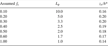
Land-cover types that exist with considerable back-ground vegetation, such as savannas, semi-deserts and shrubland, can currently be modeled using obser-vationally based assumptions and currently available NDVI and LAI databases. Provided that the total scene LAI can be obtained during a time when the grass is brown and the trees (or shrubs) are green (which can currently be determined by looking at the seasonal cycle of NDVI), the retrieved roughness length is not highly sensitive to the assumed fractional vegetation cover over a reasonable range of fc, as
il-lustrated in Table 2. For these semiarid locations, it is not unreasonable to restrict fcto between 0.1 and 0.4.
Retrievals with assumed fc ranging thus vary<20%.
The range of retrievals of zo remain within 20% for
lower assumed fractional vegetation cover (fa) in the
satellite retrieved LAI, although the retrievals with different assumed famay vary >20% (e.g. for fa=0.3,
fc=0.2 and LAI=1.0, zo/h=0.27). As Lpis related to
both the LAI and fc, Eqs. (6a), (6b), (9a) and (9b)
balance the effects of changes in assumed fc (i.e.
Eqs. (9a) and (9b) increases with increasing fc, but
Table 2
The retrieved roughness length (via Eqs. (6a), (6b), (9a) and (9b)) for an LAI of 1.0, an assumed fractional vegetation cover (fa) from the satellite of 1.0, with various assumed fractional canopy (fc) covers with a canopy aspect ratio of 1.0. The Lpis calculated via Eq. (8).
As the sensitivity to the assumed value for fc is
quite stable for the 0.2–0.3 range, a value of 0.25 is used for savannas, semi-desserts and shrublands. A maximum value for Lp is assigned to the pixel
under the conditions where the overstory is green and the understory is brown. The Lp is assumed to
decrease from these values according to seasonal-ity of satellite derived LAI. Any increases in LAI are attributed to the growth of grasses. The VCL satellite (currently scheduled for launch in Septem-ber 2000) will improve the division between trees and grasses by providing the vertical distribution of vegetation.
The largest practical limitation in applying the formulas introduced here is the uncertainty in the vegetation height, as also recognized by Jasinski and Crago who also only estimate zo/h. It may be practical
to use a correlation between albedo and vegetation height (Stanhill, 1970). However, the EDC DAAC reported albedos inferred from 1-km2 AVHRR data were found to have a low bias compared to those used by Stanhill (1970) for his correlation, and it appears desirable to include more recent data where height and albedo are both measured to establish which aldos are more credible and assess the uncertainty be-fore adjusting the correlation to the satellite albedos. The surface albedos from the moderate-resolution imaging spectroradiometer (MODIS) should be free of serious biases, but robust retrievals of canopy height on a global basis may depend on use of the VCL satellite observations that are specifically de-signed to retrieve vegetation height (among other things).
The addition of the VCL vertical vegetation distri-bution will greatly enhance the CAR retrieval, as one of the variables (hc) will be independently known.
However, initially the crown ratio is set to observa-tional values prescribed according to latitude as given in Table 1. There are indications that the roughness length and displacement height can vary depending on the leaf distribution within the crown (see Mass-man, 1997) but this information is not yet available on a global basis. The multi-angle imaging spec-troradiometer (MISR) observations may provide the crown height-to-width ratio by inversion of the sur-face brightness (a measure of the amount of shadow present) for different view directions.
While the formulas in this paper were developed in part from forest observations, they can readily be applicable to other types of land cover. The functional forms of the equations are not in question. However, there are some physiological differences between crops or grasses and forests that may make the appli-cation of these formulas more complicated. In most cases, crops (with the possible exception of corn) have a structure similar to a fully vegetated broad-leaf tree (i.e. the Lpwould be a relatively large, constant
value) and could easily be modeled. However, given that crops are usually planted in a regular pattern makes application of the formulas less reliable, be-cause at low fc values, the roughness length may
depend strongly on the wind direction. Grasslands re-quire more investigation. While it might be possible to model grass as very narrow, fully vegetated trees, the fact that grass is considerably more flexible than a tree would likely produce errors. However, retrieval errors in these short types of vegetation have a relatively small effect on global climate simulations compared to similar percentage errors in retrievals for tall vege-tation, so less accuracy may be required in crops and grassland.
5. Conclusion
This paper introduces formulas for retrieving satel-lite sensed fractional roughness length (zo/h) and
crown aspect ratio, plant leaf area index and overstory canopy height. The roughness length is a peaked func-tion in frontal area index (which is a funcfunc-tion of plant shape and spacing) and average plant LAI. The peak value of roughness length occurs between 5 and 15% fractional canopy cover for trees of typical shape. The peak roughness length in average plant LAI occurs near 0.9, which usually is seen only in the springtime green-up and fall leaf-drop. The displacement height reaches an upper limit asymptotically in both frontal area index and average plant LAI.
In many cases, the fractional vegetation cover, as currently estimated by satellite, can be used for frac-tional canopy cover. Savannas, semi-desert and shrub-land can currently be modeled with care. The crown aspect ratio is set to constant values depending on lo-cation and vegetation type. The average plant LAI is found from the satellite measured LAI in combination with the fractional vegetation cover. Both AVHRR and MODIS roughness parameters may be a significant improvement globally compared to the current fixed values used in many land/surface models.
Acknowledgements
The authors would like to N.H. Kwong for a crit-ical reading of the manuscript and M.W. Massman for many useful discussions and information. This work is made possible by the following NASA EOS Interdisciplinary Scientific Research Program grants NAG-5-4480, NAG-5-2310 and NAG-5-7249.
References
Arain, A.M., Shuttleworth, W.J., Yang, Z.-L., Michaud, J., Dolman, J., 1997. Mapping surface-cover parameters using aggregation rules and remotely sensed cover classes. Quart. J. R. Meteor. Soc. 123, 2325–2348.
Berlyn, G.P., 1962. Some size and shape relations between tree stems and crowns. Iowa St. J. Sci. 37, 7–15.
Biging, G.S., Gill, S.J., 1997. Stochastic models for conifer tree crown profiles. For. Sci. 43, 25–34.
Chen, J., Geng, X., 2000. Retrieval of boreal forest leaf area index from multiple scale remotely sensed vegetation indices, 2000. In Newcomer, J., Landis, D., Conrad, S., Curd, S., Huemmrich, K., Knapp, D., Morrell, A., Nickeson, J., Papagno, A., Rinker, D., Strub, R., Twine, T., Hall, F., Sellers, P. (Eds.), Collected Data of the Boreal Ecosystem-Atmosphere Study. CD-ROM, NASA, in press.
DeFries, R., Hansen, M., Steininger, M., Dubayah, R., Sohlberg, R., Townshend, J., 1997. Subpixel forest cover in Central Africa from multisensor, multitemporal data. Remote Sensing Environ. 60, 228–246.
Dickinson, R.E., 1983. Land surface processes and climate surface albedos and energy balance. Adv. Geophys. 25, 305–353. Dickinson, R.E., Henderson-Sellers, A., Kennedy, P.J., 1993.
Biosphere-Atmosphere Transfer Scheme (BATS) version 1e as couple to the NCAR Community Climate Model. NCAR Technical Note NCAR/TN-387+STR, Boulder, CO, 72 pp. Dickinson, R.E., Shaikh, M., Bryant, R., Graumlich, L., 1998.
Interactive canopies for a climate model. J. Clim. 11, 2823– 2836.
Eidenshink, J., Faundeen, J., 1994. The 1-km AVHRR global land set: first stages in implementation. Int. J. Remote Sensing 15, 3443–3462.
Garratt, J.R., 1994. The Atmospheric Boundary Layer. Cambridge University Press, 316 pp.
Gruszka, F., 1998. BOREAS forest cover data layers over the SSA-MSA in raster. Available online at [http://www-eosdis.ornl.gov/] from the ORNL Distributed Active Archive Center, Oak Ridge National Laboratory, Oak Ridge, TN. Halliwell, D.H., Apps, M.J., 1997. BOReal Ecosystem-Atmosphere
Study (BOREAS) biometry and auxiliary sites: overstory and understory data. Nat. Resour. Can., Can. For. Serv., North. For. Cent., Edmonton, Canada, pp 244.
Jasinski, M.F., Crago, R.D., 1999. Estimation of vegetation aerodynamic roughness of natural regions using frontal area density determined from satellite imagery. Agric. For. Meteor. 94, 65–77.
Kondo, J., Akashi, S., 1976. Numerical studies on the two-dimensional flow in horizontally homogeneous canopy layer. Agric. For. Meteor. 10, 255–272.
Lindroth, A., 1993. Aerodynamic and canopy resistance of short-rotation forest in relationship to leaf area index and climate. Bound.-Layer Meteor. 66, 265–279.
MaGuire, D.A., Hann, D.W., 1989. The relationship between gross crown dimensions and sapwood area at crown base in Douglas-Fir. Can. J. For. Res. 19, 557–565.
Massman, W.J., 1997. An analytical one-dimensional model of momentum transfer by vegetation of arbitrary structure. Bound.-Layer Meteor. 83, 407–421.
Myneni, R.B., Nemani, R.R., Running, S.W., 1997. Estimation of global Leaf Area Index and absorbed Par using radiative transfer models. IEEE Trans. Geo. Remote Sensing 35, 1380–1393. Pitman, A.J., 1994. Assessing the sensitivity of a land-surface
scheme to the parameter values using a single column model. J. Clim. Meteor. 7, 1856–1869.
Raupach, M.R., 1992. Drag and drag partition on rough surfaces. Bound.-Layer Meteor. 60, 375–395.
Raupach, M.R., 1994. Simplified expressions for vegetation roughness length and zero-plane displacement as a function of canopy height and area index. Bound.-Layer Meteor. 71, 211–216.
Seginer, I., 1974. Aerodynamic roughness of vegetated surfaces. Bound.-Layer Meteor. 5, 383–393.
revised land surface parameterization (SiB2) for atmospheric GCMs: Part 1: Model formulation. J. Clim. 9, 676–737. Shaw, R.H., Pereira, A.R., 1982. Aerodynamic roughness of a
plant canopy: a numerical experiment. Agric. Meteorol. 26, 51–65.
Schaudt, K.J., 1998. A new method for estimating roughness parameters and evaluating the quality of observations. J. Appl. Meteor. 37, 470–476.
Stanhill, G., 1970. Some results of helicopter measurements of the albedo of different land surfaces. Solar Energy 66, 59–66. Thom, A.S., 1975. Vegetation and the Atmosphere, Principles, Vol.
1, Academic Press, 278 pp.