A COMPARISON OF UAV AND TLS DATA FOR SOIL ROUGHNESS ASSESSMENT
M. Milenkovi´ca,∗, W. Karela, C. Ressla, N. Pfeifera,
aDept. of Geodesy and Geoinformation, Vienna University of Technology, Gußhausstraße 27-29, 1040 Vienna, Austria (Milutin.Milenkovic, Wilfried.Karel, Camillo.Ressl, Norbert.Pfeifer)@geo.tuwien.ac.at
Commission V, WG V/5
KEY WORDS:Autocorrelation function, Correlation length, Power spectral density, Fractal dimension, Error propagation, Bundle adjustment
ABSTRACT:
Soil roughness represents fine-scale surface geometry which figures in many geophysical models. While static photogrammetric tech-niques (terrestrial images and laser scanning) have been recently proposed as a new source for deriving roughness heights, there is still need to overcome acquisition scale and viewing geometry issues. By contrast to the static techniques, images taken from unmanned aerial vehicles (UAV) can maintain near-nadir looking geometry over scales of several agricultural fields. This paper presents a pilot study on high-resolution, soil roughness reconstruction and assessment from UAV images over an agricultural plot. As a reference method, terrestrial laser scanning (TLS) was applied on a 10 m x 1.5 m subplot. The UAV images were self-calibrated and oriented within a bundle adjustment, and processed further up to a dense-matched digital surface model (DSM). The analysis of the UAV- and TLS-DSMs were performed in the spatial domain based on the surface autocorrelation function and the correlation length, and in the frequency domain based on the roughness spectrum and the surface fractal dimension (spectral slope). The TLS- and UAV-DSM dif-ferences were found to be under±1 cm, while the UAV DSM showed a systematic pattern below this scale, which was explained by weakly tied sub-blocks of the bundle block. The results also confirmed that the existing TLS methods leads to roughness assessment up to 5 mm resolution. However, for our UAV data, this was not possible to achieve, though it was shown that for spatial scales of 12 cm and larger, both methods appear to be usable. Additionally, this paper suggests a method to propagate measurement errors to the correlation length.
1. INTRODUCTION
Roughness is a property of surfaces, required to understand and model interaction at these surfaces, e.g. in hydraulics, radar re-mote sensing, or soil erosion. The assessment of roughness has been traditionally performed by mechanical profiling (Mattia et al., 2003), but this is naturally restricted by the length of the ruler and the effort to place it at different locations. With effi-cient methods for acquiring point clouds at high resolution like terrestrial laser scanning (TLS) and high density image match-ing (Lichti and Jamtsho, 2006) (Rothermel et al., 2012) (Rieke-Zapp and Nearing, 2005), new possibilities for assessing rough-ness arise. The range envelope for which roughrough-ness should be quantified depends on the application. In radar remote sensing, but likewise in the optical domain, the backscattering behavior depends on the roughness in relation to the wavelength (Ulaby et al., 1986). As an example, Sentinel-1 has a wavelength of 5.5 cm. Thus, the roughness between a few mm and up to several decimeters should be modeled.
The shape of a rough surface can be modeled as a random pro-cess, as a scalar function of the X- and Y-coordinate (Verhoest et al., 2008). Assessing the roughness therefore requires the study of a larger area. Using again the example of Sentinel-1, which has a resolution of 5 m x 20 m, a highly detailed surface model should be derived for an extent of several multiples of 20 m.
Terrestrial laser scanning has proven to be a suitable tool for mod-eling the roughness at the required scales. Positioning the TLS at large height above the ground, and restricting the ranges used, guarantees that roughness content placed close to the Nyquist fre-quency is assessed with 5% accuracy or better (Milenkovi´c et al.,
∗Corresponding author
2015). However, for larger areas this procedure is less practica-ble due to the number of required stand points. Airborne acqui-sition, in contrast, allows large area coverage. However, standard photogrammetric flights cannot provide the resolution required. Lower flying heights would be necessary to reach it.
Using a UAV these low flying heights become possible: the air-borne close range approach. Above that, low cost components (small UAVs, consumer cameras), make this approach interest-ing. However, little work has been performed on very high res-olution mapping of irregular surfaces by UAVs. In (Eltner et al., 2013), UAV images with 2-4 mm ground sampling distance (GSD) were used to provide cm to sub-cm accurate DSMs for multi-temporal soil erosion monitoring. Also (Mancini et al., 2013) reported that UAV data with 6 mm resolution was acquired to monitor beach dune geometry. The heights reconstructed from this UAV data were within a few centimeters compared to the heights of a TLS data set used as the reference.
The aim of this article is to investigate if the quality obtained by TLS can be achieved also by light weight UAV image based acquisition. Specifically, in this paper data is acquired over a plot of bare soil, by TLS and with images from a UAV. The surface model from TLS serves as a reference and the model from the images is compared against it. This comparison is performed on the basis of roughness measures.
2. EXPERIMENT SETUP AND DATA
2.1 Experiment Setup
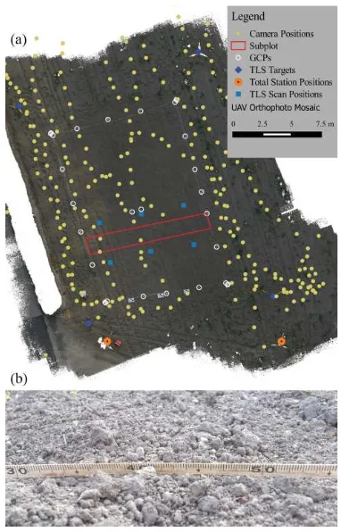
Figure 1: (a) The agricultural plot with the UAV and TLS mea-surement setup; (b) An image of the fine-scale roughness ele-ments present in the plot.
June 2015. The weather was mostly sunny with some short cloud interruptions and without rain, but with wind that was strong enough to prevent the UAV from flying in autopilot mode.
The experimental setup is shown in Figure 1a, where the or-thophoto derived from the UAV images was used as background. The large rectangular plot delineated by the ground control points (GCPs, the white circles in Figure 1a) was surveyed with the UAV images, while a subplot of ca. 10 m x 1.5 m (the red rectangle) was surveyed with the TLS. Additionally, total station measure-ments were performed to define a local datum, i.e. to derive co-ordinates of the GCPs in the local object coordinate system. The GCPs were symmetrically distributed around the plot and sepa-rated at maximum 3 m from one another. This, rather small, GCP spacing was selected to minimize systematic deformations in the object space due to residual errors in the images.
The agricultural soil plot contained roughness elements over sev-eral scales. The most prominent ones were low-frequency peri-odic surface components (2 to 3 cm in the amplitude) which were introduced with a mechanical, seed-bed preparation tool. On top of these components, there were randomly distributed soil clods (soil aggregates up to a few centimeters), very fine soil grains (Figure 1b), and a number of small, individual vegetation patches (up to a few decimeters). Since the purpose of this study was to characterize the bare soil roughness, this vegetation was removed from the plot before data acquisition.
2.2 UAV Images
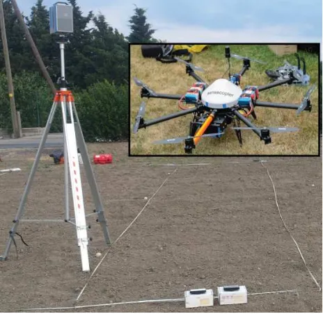
The images were collected with a SonyαILCE-6000, an inter-changeable lens camera mounted on an octocopter (Figure 4). The camera’s sensor size is 23.5 mm x 15.6 mm, which corre-sponds to pixel size of 3.9µm. The camera was combined with a
Figure 2: (a) Image density map (the GCPs are plotted as red dots); (b) Image footprints within the subplot.
zoom lens Sony AF E 16-70mm 4.0 ZA OSS, the focal length of which was 52 mm during image acquisition.
Due to strong wind, the flight was performed manually and as much as possible parallel to the two longer sides of the plot. The flight took 13 minutes to acquire 254 images, which were pre-dominately distributed along the two longer sides of the plot, but with some of them also distributed along the plot’s central axis (Figure 1). Thus, the acquired images were not distributed in the well-know regular strip pattern. Nevertheless, as shown in Fig-ure 2a, the plot was covered everywhere with at least 9 images. The average flying height was 22 m, which resulted in a ground sampling distance (GSD) below 2 mm. The images were self-calibrated in a bundle block adjustment procedure.
The image resolution was then examined based on the edge spread function, also known as edge response (Perko et al., 2004)(Ja-cobsen, 2009). The edge spread function was calculated by the QuickMTF software (www.quickmtf.com) using the special test charts (provided by the software company) which were printed and fixed to flat plates on the ground during image acquisition (Figure 3a-b). The estimated modulation transfer functions for each color are shown in Figure 3. According to the 50 % modu-lation threshold, the reported resolution is 6 pixels, which is ap-proximately 12 mm in the object space. This resolution is notably lower compared to the images’ GSD (ca. 2 mm). One of the rea-sons for this degradation of image resolution is motion blur which is most probably caused by an inappropriate shutter time setting and vibration of the UAV.
2.3 TLS Data
Figure 3: The modulation transfer function (MTF) corresponding to the edge spread function (measured in the in-flight direction) of an acquired image.
taken from classical geodetic tripods. However, UAV images are collected in a kinetic mode,which degrades the resolution by sev-eral pixels due to motion blur. On the other hand, the scanner itself is static and a single measurement takes less than one micro-second. Moreover, the TLS was applied here from a high tripod (instrument height>2.5m) and with small ranges (<6 m), which provided more favorable viewing geometry and higher resolution compared to classical TLS setups and our UAV data.
2.3.1 Measurement Setup The subplot was scanned with 6 scan positions in total, where 3 of them were taken along each of the two longer sides of the subplot. To minimize occlusions and incidence angles, the scan positions were set approximately opposite to one another and the scanner was placed on a high tripod (Figure 4). The instrument height ranged from 2.55 m to 2.72 m. Scanning was performed in the quality and high-sampling mode, providing 10000 range measurements per full circle. The scanning started at 19:10 CET and completed in 50 minutes, taking on average 9 minutes per station.
The TLS points collected within the subplot have the following characteristics. 95 % of the points have a range smaller than 4.5 m. Since the scanner has a precise laser beam (3 mm beam diam-eter at the exit and a divergence of 0.3 mrad), the diamdiam-eter of the laser-beam footprint was below 5 mm all over the subplot. 90% of the points have an incidence angle below 52◦, which fulfills the requirements suggested by (Milenkovi´c et al., 2015) for TLS in roughness applications. The average point density within the subplot is 85 points/m2
, while 90% of the subplot has at least 40 points/m2
, i.e. the point spacing within the subplot is 1.5 mm or smaller. This means that the laser-beam footprints of neighboring points were overlapping one another, which is also known as the correlated sampling mode where the resolution of the TLS data is rather limited by the laser beam footprint (Lichti and Jamtsho, 2006) and (Milenkovi´c et al., 2015). This means that the resolu-tion of this TLS data is approximately 5 mm.
2.3.2 TLS Data Pre-Processing The six raw TLS scans were first preprocessed in “Z + F Laser Control”software where the mixed-pixel and single-pixel filters were applied. These filters
remove points with erroneous range values happened when the laser beam of a phase-comparison laser scanner illuminates sev-eral objects distributed along the laser line of sight (Langer et al., 2000). For our surface, this mostly happened when the laser beam simultaneously illuminated the top of a soil clod and the soil surface in the background. In addition to these filters, the inten-sity filter was applied to remove points with an inteninten-sity smaller than 1 %. These points are generally less accurate because their range determination is associated with a small signal to noise ra-tio (Langer et al., 2000).
The parameter values used in the above filters (mixed-pixel, single-pixel and intensity) are the default values recommended by the “Z + F Laser Control” software. This default parameter setting was already found to be appropriate for soil-roughness preprocessing (Milenkovi´c et al., 2015).
3. METHODS
3.1 UAV Data Processing
The UAV imagery was oriented and the camera was calibrated using OrientAL (Karel et al., 2013). Missing any direct sensor orientation data, processing started with a variation of Structure-from-Motion (SfM) (Torr and Zisserman, 2000): image feature points are detected in each image and their neighborhoods are described, after which point pairs with similar descriptors are matched between image pairs. Relative image pair orientations are computed and outlier matches discarded. For an initial im-age pair, object points are forward intersected and both camera orientations and object points are optimized in a bundle block ad-justment. Subsequently, additional images are added to the block one after another by spatial resection and further object points are triangulated, until all images have been oriented. Aiming at the error-free and precise orientation of all images, robust methods are employed at all stages, and intermediate bundle block adjust-ments are executed after the addition of further images. Already the pairwise image matching takes place in Euclidean space, us-ing an approximate interior orientation derived from Exif data. In contrast to other software packages, OrientAL estimates a vari-able set of lens distortion parameters, depending on their
icance and stability, and to better handle perspective image dis-tortion, we use Affine SIFT features (Morel and G.Yu, 2009), which are not only scale and rotation invariant, but also invari-ant to affine distortion. Finally, the maximum admissible image point residual norm is not a fixed parameter, but is derived from the data itself.
Using these relative image orientations, we forward intersect the GCPs into model space using their manual image observations, apply the resulting similarity transform to the bundle block, and introduce additional observations for the GCPs in image and ob-ject space, taking into account their stochastic nature. While we assumed the standard deviations of feature point image observa-tions a priori to be 1 pix, image observaobserva-tions of control points were given the higher precision of 0.1 pix due to their higher definition accuracy. Observations of control point coordinates in object space were assigned a standard deviation of 1 mm a priori. This resulted in median residual norms for feature image points of 0.46 pix, for GCP image points of 0.97 pix, and for GCP object points of 14 mm. The rather large residuals of GCP image points may be a result of the weak block geometry with 2 flight strips of extremely high overlap along-track, but low overlap across-track.
3.2 Data Co-Registration
Before interpolation and data comparison, it was necessary to bring the UAV and TLS data into the same local object coordi-nate system (LOCS). This was done trough several co-registration steps. First, the individual TLS scans were georeferenced to the LOCS with the help of the control points measured with the total station. This procedure was performed using an adjustment pro-cedure implemented in “Z + F Laser Control” software. Then, in an additional step, the individual TLS scans were co-registered to one another using a variant of the iterative closest point (ICP) al-gorithm implemented in the software OPALS (Glira et al., 2015). This step minimizes the point-to-surface distance among all the scans, and for our 6 scans data, the standard deviation of this dis-tance after the ICP procedure was 0.8 mm. This value is just two times the specified measurement noise of the Z + F IMAGER 5010c scanner, which suggests at very good co-registration of the TLS scans. The six TLS scans were then merged into one TLS point-cloud block.
The UAV images were oriented trough a bundle adjustment pro-cedure where the GCP coordinates measured with the total station were also used as observations. Thus, the resulting exterior cam-era parameters were already in the LOCS. This means that the densely matched points as well as the automatically derived UAV DSM are both in the LOCS. Still, in order to remove any remain-ing residual errors in the absolute orientation and to optimize the relative orientation between UAV DSM and TLS DSM, another ICP run was applied to both DSMs. The standard deviation of the final point-to-surface distances between UAV DSM and the TLS block was 4 mm.
3.3 Detrending and DSM Interpolation
Roughness analysis is generally performed on detrended heights. Thus, the UAV and TLS data were additionally detrended here using the regression plane fitted trough the TLS points within the subplot. This means that the detrended UAV and TLS heights were calculated as the normal residuals to the regression plane, while the planar coordinates were additionally reduced to the cen-ter of gravity of the TLS points.
The TLS DSM was interpolated from the detrended TLS point-cloud block. The interpolation was done for a 1 mm grid spacing
and with the moving plane interpolation applied to points within a 2.5 mm neighborhood radius. This neighborhood size was se-lected to match the size of the laser beam footprint within the plot. The UAV DSM was automatically produced by the SURE software (Rothermel et al., 2012), where the bundle results were supplied as input.
3.4 Roughness Assessment
Surface roughness is treated here in two ways: (a) through the so-called classical parametrization, i.e. as a zero-mean Gaussian process characterized by the root mean square (RMS) height, autocorrelation function (ACF) and correlation length (l) (Ver-hoest et al., 2008), and (b) as a band-limited random fractal sur-face characterized by the spectral slope (α), i.e. fractal dimen-sionD = 5−α
2 (Davidson et al., 2003). Both parametrizations were estimated as in (Milenkovi´c et al., 2015), i.e. from linearly-detrended soil-roughness profiles sampled as rows of the TLS and UAV DSMs.
For the classical parametrization, first the empirical autocorrela-tion funcautocorrela-tion was derived, with its value for a lagτkcalculated as: the DSM’s grid size.Nis the number of height samples in a DSM row, whileziandzi+k are the DSM row heights at positionsi and i+k, respectively. The RMS height s was estimated as s2
= ˆr(0), while the correlation lengthlwas calculated as in (Davidson et al., 2003), i.e. directly interpolating the normalized autocorrelation functionρ(τk) = ˆr(τk)/ˆr(0):
For the fractal parametrization, it was necessary first to estimate the power spectral density (the roughness spectra). This was done by calculating the assembly-average of the hamming-windowed periodograms derived from the sampled DSM rows (Milenkovi´c et al., 2015). Based on the derived roughness spectra, the spec-tral slopeαis calculated as the slope of a regression line used to approximate the roughness spectrum on the logarithmic scale and within a particular frequency band (Dierking, 1999). In the linear-scale frequency domain, the latter is equivalent to:
S(f) =c·f−α
(3)
wherefis the spatial frequency,log10(c)is the intercept of the regression line, andS(f)is the roughness spectrum.
3.4.1 Roughness Levels of Detail The roughness level of de-tail present in the TLS- and UAV-DSM is judged in two ways: (a) qualitatively, by visual comparison of the DSMs’ shaded models, and (b) quantitatively, by calculating the difference of the esti-mated UAV and TLS roughness spectra. The roughness spectra difference can reveal the spatial wavelengths (scales) over which two corresponding DSMs share the same roughness information. According to the study of (Oh and Kay, 1998), which is based on synthetic data, the roughness spectra difference should be be-low 1 dB for accurate prediction of the microwave backscatter strength.
3.5 Autocorrelation Function and Error Propagation
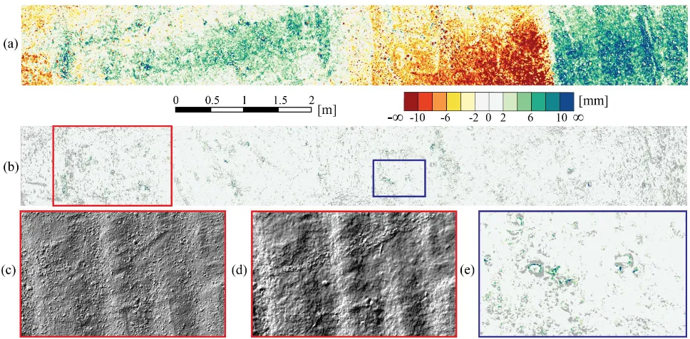
inter-Figure 5: (a) Difference map between the TLS- and the UAV-DSM; (b) Min-max distance map derived from the DSMs of six overlap-ping single-TLS scans; (c) and (d) are shaded TLS- and UAV-DSM, respectively, from the region marked by the red rectangle in (b); (e) is the zoom-in to the blue rectangle in (b).
polation errors. Thus, this section considers how these errors can be quantified and propagated further to to the autocorrelation es-timates.
For the TLS DSM, the height errors are quantified with the moving-plane interpolation errorσz. This error is derived for each grid position by propagating the RMS error of the plane adjustment procedure of the neighboring points during the interpolation pro-cess. Since the neighborhood used in our case is small (2.5 mm radius), the interpolation error can be seen as a mixture of the measurement noise as well as the modeling error caused by a pla-nar approximation of roughness elements like soil clods.
For the UAV DSM, the height error is quantified as the standard deviation (σM AD) derived from the median of absolute differ-ences of the dense-matched point’s heights within 6 mm neigh-borhood radius. The dense-matched points are one of the outputs provided by SURE, and they are calculated while matching a base image with several neighboring images (Rothermel et al., 2012). This means that for each pixel of a base image there are sev-eral reconstructed heights corresponding to the neighboring im-age pairs. Therefore, the DSM heights (also provided by SURE) can be seen as a median-like filter of the matched points. The σM ADestimation radius (6 mm) was set according to the image resolution in the object space (ca. 12 mm).
σz andσM AD are available for each height of the TLS DSM and UAV DSM, respectively. Based on Eq.(1), it is possible to propagateσzandσM ADfurther to the autocorrelation values for each particular lag. This can be easily done when Eq.(1) is seen as linear combination, i.e. as a product of a row vectorh⊤k and a column vectorz:
ˆ r(τk) =
1 N−k
N−k
X
i=1
zizi+k=h⊤k ·z, (4)
where:
hk= 1 N−k
0
z1 .. . zN−k
,and z=
z1 z2 .. . zN
,
while the firstkelements ofhkare zeros. For the zero-lag auto-correlationˆr(0), it holds:h0 = 1
Nz. Following the error prop-agation law forhkandz(both contain individual random vari-ables), the expression for the variance of a single-lag autocorre-lation valuer(τˆ k)is:
ˆ σr2k =h
⊤
k ·Σzz·hk+zk⊤·Σhkhk·zk (5)
Σzz is a full diagonal matrix containing variances σ2 zi, while Σhkhkis the same asΣzz, but with the first k diagonal elements
equal to zero. Finally, to compute the variance ofr(τˆ k)for the TLS DSM, theσ2
zi values are replaced withσ
2
z, while in case of the UAV DSM, theσ2
M ADis used instead.
4. RESULTS AND ANALYSIS
4.1 Accuracy of Data Co-Registration
Improper data co-registration may lead to false roughness analy-sis. Thus, two elevation-difference rasters were prepared to report on the co-registration accuracy: one to check the co-registration of the individual TLS scans, and another to check the co-registration of the TLS DSM and UAV DSM.
areas which contain just one individual TLS DSM, and they oc-cupy about 30% of the plot. The 95% of the remaining area con-tains range values below 2 mm, which indicates a very good co-registration of the TLS scans. The remaining 5% of large range values occurs mostly around the soil clod edges, which can be seen in Figure 5e. This is because the moving-plane interpolation with a neighborhood radius of 2.5 mm (the interpolation method used for the DSM interpolation) does not perform well on soil clod borders. However, these are generally known interpolation artifacts that can not be easily overcome with our TLS data.
Figure 5a shows the color-coded elevation differences between the UAV DSM and the TLS DSM. Due to the ICP minimization between the two DSMs performed in the preprocessing step, the differences are on average zero, and 90% of the differences are within±9 mm. However, within this accuracy range, there are also large systematic patterns in the difference map. After careful examination, it was found that borders between regions of posi-tive and negaposi-tive differences correspond to image borders (see Figure 2b). Residual image orientation errors may be responsible for that. These orientation errors could be caused by insufficient overlap between individual image sub-blocks. Additionally, dur-ing the image acquisition, the image stabilization was switched on to reduce motion blur, which caused unstable inner geometry of the camera, and consequently, difficulties to determine a sin-gle distortion model valid for all images. With an accuracy of
±9 mm this UAV DSM is only sub-optimal. Still, within this accuracy bound, the UAV DSM can be used for the comparison with the TLS DSM. However, this experience raises the aware-ness that the acquisition of the UAV images should be conducted with much more care - especially regarding the stability of the in-ner image geometry. For an identical image set with a stable inin-ner geometry, the accuracy of the UAV DSM should be expected to be notably higher, and without the systematic effects shown in Figure 5a.
4.2 Roughness Assessment in Frequency Domain
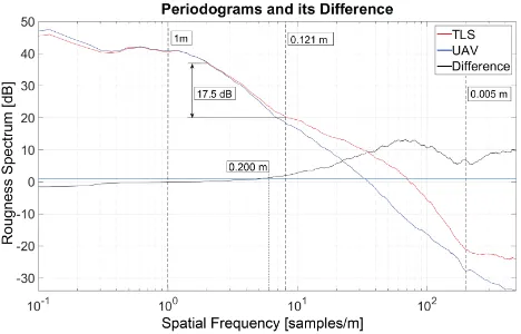
The TLS and UAV DSMs of the whole plot are analyzed here in the frequency domain. Figure 6 shows two roughness spectrum lines derived from the TLS DSM (red) and UAV DSM (blue), re-spectively. They are the ensemble-average, hamming-windowed periodograms derived from 100 rows of the corresponding DSMs. To make interpretation easier, the periodograms were further smo-othed with the moving average with the span of 100 elements. This procedure preserves the general trend of the periodogram while removing the undesirable variability associated with this estimator. The black line in Figure 6 shows the difference be-tween the TLS- and UAV-based periodograms.
There are 4 frequency bands where the roughness spectra per-form differently. These bands are separated with the three vertical dashed lines in Figure 6. The very right band (from the Nyquist up to the 5 mm wavelength) of the TLS spectrum shows a white-noise (horizontal) roll-off, indicating that there is no further infor-mation contained. This is fully consistent with the resolution of the TLS DSM, i.e. with the diameter of the laser footprint which was up to 5 mm within the subplot. These frequencies are present in the periodogram because the TLS DSM was unnecessarily in-terpolated to 1 mm grid even though the resolution of the data itself was lower (5 mm). However, this was performed just to have an additional estimate of the resolution of our control data set, and to illustrate that the Nyquist frequency does not neces-sarily indicate the resolution of a DSM. Additionally, it can be seen that the roughness spectrum at these frequencies is below -20 dB, which is several orders of magnitude smaller than the TLS measurement noise. This indicates that the measurement noise is
Figure 6: The PSD functions
filtered out from the TLS point cloud during the DSM interpola-tion. Thus, it shows that the TLS data are appropriately modeled.
From the spectra difference, it can be shown that the roughness spectra are similar in the first two frequency bands up to the 1 dB limit (the blue horizontal line in Figure 6). The 1 dB limit was selected according to a study of (Oh and Kay, 1998). This prac-tically means that the TLS DSM can be readily replaced with the UAV DSM when the relevant roughness content is placed along wavelengths up to 20 cm. For shorter wavelengths (from 20 cm till 5 mm), the TLS roughness spectrum contains much more roughness information than the UAV spectrum. This can be also seen in the two shaded DSMs (Figure 5c and 5d), which clearly show that the TLS DSM contains much more roughness elements at these scales compared with the UAV DSM, where they are smoothed out. The latter effect is most probably a conse-quence of image resolution and orientation errors which directly influence the DSM.
In the second frequency band (from 1 m to 12 cm wavelengths), both spectra exhibit a linear (fractal) nature, while the power of the UAV DSM drops faster (17.5 dB per 0.5 of decade) compared with the TLS power drop (17.5 dB per 0.6 of decade). The latter is equivalent to the spectral slope values of 3.5 and 2.6 for the UAV- and TLS-DSM, respectively. Thus, in this frequency band, the UAV DSM has a slightly higher spectral slope (smaller fractal dimension) compared with the TLS DSM. This shows that even though the underlying surface is identical for both data sets, the UAV and TLS data suggest two families of surfaces with different stochastic properties. This, in turn, may cause an inconsistent prediction of the microwave backscatter energy from the same surface.
Finally, in the very left frequency band (from DC till 1 m wave-length), the UAV spectrum is on top of the TLS spectrum, which is opposite to its behavior along the remaining frequencies. This shows that UAV spectra has more power at these frequencies compared with the TLS DSM, which is a consequence of the sys-tematics present in the UAV DSM (Figure 5a).
4.3 Roughness Assessment in Spatial Domain
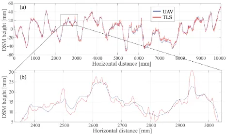
Figure 7: (a) Single TLS and UAV height profiles sampled at identical location from the corresponding DSMs; (b) Zoom-in to portions of the profiles in (a).
are completely smoothed out in the UAV profile (e.g. section from 2.6 m to 2.7 m, Figure 7b). However, due to the systematic errors in the UAV DSM, this did not have an effect on the profiles’ RMS height values, where the RMS height of the UAV profile (suav= 22mm) was found even larger than the RMS height (stls = 20 mm) of the TLS profile.
The correlation length, as a measure of roughness, was deter-mined for both data sets. As can be seen in Figure 8 the shapes of the autocorrelation functions are similar, and the faster drop was explained as result of the finer details visible in the TLS data. The correlation length determined from the UAV images is thus approximately 15% larger than for the TLS data. In this article error propagation was used to forward the uncertainty of eleva-tion to uncertainty of the autocorrelaeleva-tion funceleva-tion and further to the precision of the estimated correlation length. Given the lower accuracy of the image based surface model, the precision of the corresponding correlation length is poorer, too, but still only a few percent of the correlation length. This uncertainty is much lower than the offset in correlation length between the two meth-ods. This suggests, that this error estimate is too optimistic, and a likely cause is that correlations between the individual elevation measures remained unconsidered (diagonal matrix in Eq (5)).
5. DISCUSSION AND CONCLUSIONS
In this experiment, a UAV data set was analyzed for soil rough-ness assessment. The images used in the experiment had a resolu-tion of 12 mm, which is low compared to the GSD of 2 mm. The reason was the motion blur and poor lighting conditions, which led to a loss of sharpness at the individual pixel level. Terrestrial laser scanning was used as a reference method here, which does not suffer from these two effects.
Although in this experiment the TLS was selected as the refer-ence, point clouds based on overlapping images taken very close to the object and using static acquisition can be more accurate. For example, the vertical accuracy and GSD of an image block taken 1 m apart from the object and with a contemporary cam-era and a normal-angle lens, can be a few tenths of mm (Kraus, 2007). This is notably better than the TLS co-registration accu-racy and the laser footprint, both found here to be of a few mm. Thus, in further experiments, static and very close-range overlap-ping imaging can be considered as the reference as well.
In Figure 5a systematic errors in the surface model derived from dense image matching became apparent, under the assumption that the TLS data serves as reference. That these systematic errors
Figure 8: Normalized autocorrelation functions based on the TLS DSM and UAV DSM. The red dashed lines shows the 3σbounds of the propagated errors.
are related to the bundle block adjustment or the dense matching is further supported by the comparison of the pattern of Figure 5a to Figure 2b, which shows the overlap as grey tone and the image borders. Changes from negative to positive errors occur at regions where the overlap strongly drops. Thus, we conclude that images within the bundle formed a sub-block which has strong ties within itself, but poorer ties to neighboring sub-blocks. In this context it is noted that clods and soil grains may look differently from different perspectives, e.g. due to cast shadow, near vertical ele-ments, etc. This would introduce high correlation between some images, which is not considered in the stochastic model of the bundle block adjustment used here.
Based on the performed analysis, one conclusion is that obtain-ing very high resolution images of natural bare soil surfaces with UAV remains challenging with low-cost components. The stabil-ity of the camera is of concern, which can be enhanced (turning off auto-focus, stabilizer, etc.) with suitable cameras. However, the limited stability of consumer cameras is generally known. Secondly, flying has to support image acquisition, thus avoiding motion blur due to forward motion or vibrations. Additionally, the experiment suggests that a regular block layout of the images within the block could prevent systematic errors due to forming of sub-blocks within the bundle block adjustment.
The experiment uses the methods suggested in (Milenkovi´c et al., 2015) for processing TLS data to assess surface roughness. The results are consistent with the previous study, and thus, confirm the suggested method and show that it is extendable for TLS data taken from high tripods and over a larger area. We could not prove that the low-cost UAV images considered in this experi-ment can deliver the same level of detail and accuracy as current TLS systems (resolution of 5mm), although improvement can be expected. However, for spatial scales of 12cm and larger (Figure 6), both methods appear to be usable.
use them in synergy.
ACKNOWLEDGEMENTS
The research leading to these results has received funding from the European Community’s Seventh Framework Programme ([ FP7 / 2007 - 2013 ]) under grant agreement no 606971.
We would also like to thank Melanie Raˇskovi´c for helping with measurements of the ground control points as well as Peter Dorni-nger and Clemens Nothegger from 4D-IT GmbH for collecting the UAV images.
REFERENCES
Davidson, M., Mattia, F., Satalino, G., Verhoest, N., Le Toan, T., Borgeaud, M., Louis, J. and Attema, E., 2003. Joint statisti-cal properties of rms height and correlation length derived from multisite 1-m roughness measurements. Geoscience and Remote Sensing, IEEE Transactions on 41(7), pp. 1651–1658.
Dierking, W., 1999. Quantitative roughness characterization of geological surfaces and implications for radar signature analysis. Geoscience and Remote Sensing, IEEE Transactions on 37(5), pp. 2397–2412.
Eltner, A., Mulsow, C. and Maas, H.-G., 2013. Quantitative mea-surement of soil erosion from tls and uav data. ISPRS - Inter-national Archives of the Photogrammetry, Remote Sensing and Spatial Information Sciences XL-1/W2, pp. 119–124.
Glira, P., Pfeifer, N., Briese, C. and Ressl, C., 2015. A corre-spondence framework for als strip adjustments based on variants of the icp algorithm. Photogrammetrie - Fernerkundung - Geoin-formation 2015(4), pp. 275–289.
Jacobsen, K., 2009. Effective resolution of digital frame images. In: International Archives of the Photogrammetry, Remote Sens-ing and Spatial Information Sciences.
Karel, W., Doneus, M., Verhoeven, G., Briese, C., Ressl, C. and Pfeifer, N., 2013. Oriental - automatic geo-referencing and ortho-rectification of archeological aerial photographs. In: ISPRS An-nals of the Photogrammetry, Remote Sensing and Spatial Infor-mation Sciences, II-5/W1.
Kraus, K., 2007. Photogrammetry – Geometry from Images and Laser Scans. 2 edn, De Gruyter.
Langer, D., Mettenleiter, M., H¨artl, F. and Fr¨ohlich, C., 2000. Imaging ladar for 3-d surveying and cad modeling of real-world environments. The International Journal of Robotics Research 19(11), pp. 1075–1088.
Lichti, D. D. and Jamtsho, S., 2006. Angular resolution of ter-restrial laser scanners. The Photogrammetric Record 21(114), pp. 141–160.
Mancini, F., Dubbini, M., Gattelli, M., Stecchi, F., Fabbri, S. and Gabbianelli, G., 2013. Using unmanned aerial vehicles (uav) for high-resolution reconstruction of topography: The structure from motion approach on coastal environments. Remote Sensing 5(12), pp. 6880.
Mattia, F., Davidson, M., Le Toan, T., D’Haese, C., Verhoest, N., Gatti, A. and Borgeaud, M., 2003. A comparison between soil roughness statistics used in surface scattering models derived from mechanical and laser profilers. Geoscience and Remote Sensing, IEEE Transactions on 41(7), pp. 1659–1671.
Milenkovi´c, M., Pfeifer, N. and Glira, P., 2015. Applying terres-trial laser scanning for soil surface roughness assessment. Re-mote Sensing 7(2), pp. 2007.
Morel, J. and G.Yu, 2009. ASIFT: A new framework for fully affine invariant image comparison. SIAM Journal on Imaging Sciences.
Oh, Y. and Kay, Y. C., 1998. Condition for precise measurement of soil surface roughness. Geoscience and Remote Sensing, IEEE Transactions on 36(2), pp. 691–695.
Perko, R., Klaus, A. and Gruber, M., 2004. Quality comparison of digital and film-based images for photogrammetric purposes. In: International Archives of Photogrammetry, Remote Sensing and Spatial Information Sciences.
Rieke-Zapp, D. H. and Nearing, M. A., 2005. Digital close range photogrammetry for measurement of soil erosion. The Pho-togrammetric Record 20(109), pp. 69–87.
Rothermel, M., Wenzel, K., Fritsch, D. and Haala, N., 2012. SURE: Photogrammetric surface reconstruction from imagery. In: Proceedings LC3D Workshop, Berlin, December 2012.
Torr, P. H. and Zisserman, A., 2000. Feature based methods for structure and motion estimation. In: Vision Algorithms: Theory and Practice, Springer, pp. 278–294.
Ulaby, F., Moore, R. and Fung, A., 1986. Microwave Re-mote Sensing: Active and Passive. Artech House microwave library, Addison-Wesley Publishing Company, Advanced Book Program/World Science Division.