IMPROVING 3D SPATIAL QUERIES SEARCH: NEWFANGLED TECHNIQUE OF SPACE
FILLING CURVES IN 3D CITY MODELING
U. Uznira
Dept. of Geoinformation, Faculty of Geoinformation and Real Estate, Universiti Teknologi Malaysia, 81310 Skudai, Johor, Malaysia
[email protected], [email protected], [email protected] b
Dept. of Geodesy, National Space Institute, Denmark Technical University, 2800 Lyngby, Denmark {fa,mioc}@space.dtu.dk
Commission II WG II/2
KEY WORDS:3D Spatial Data Management, 3D Space Filling Curves, 3D City Modeling, 3D Adjacency, 3D Indexing
ABSTRACT:
The advantages of three dimensional (3D) city models can be seen in various applications including photogrammetry, urban and regional planning, computer games, etc.. They expand the visualization and analysis capabilities of Geographic Information Systems on cities, and they can be developed using web standards. However, these 3D city models consume much more storage compared to two dimensional (2D) spatial data. They involve extra geometrical and topological information together with semantic data. Without a proper spatial data clustering method and its corresponding spatial data access method, retrieving portions of and especially searching these 3D city models, will not be done optimally. Even though current developments are based on an open data model allotted by the Open Geospatial Consortium (OGC) called CityGML, its XML-based structure makes it challenging to cluster the 3D urban objects. In this research, we propose an opponent data constellation technique of space-filling curves (3D Hilbert curves) for 3D city model data representation. Unlike previous methods, that try to project 3D or n-dimensional data down to 2D or 3D using Principal Component Analysis (PCA) or Hilbert mappings, in this research, we extend the Hilbert space-filling curve to one higher dimension for 3D city model data implementations. The query performance was tested using a CityGML dataset of 1,000 building blocks and the results are presented in this paper. The advantages of implementing space-filling curves in 3D city modeling will improve data retrieval time by means of optimized 3D adjacency, nearest neighbor information and 3D indexing. The Hilbert mapping, which maps a sub-interval of the[0,1]interval to the corresponding portion of the d-dimensional Hilbert’s curve, preserves the Lebesgue measure and is Lipschitz continuous. Depending on the applications, several alternatives are possible in order to cluster spatial data together in the third dimension compared to its clustering in 2D.
1 INTRODUCTION
3D spatial city models in different applications require different analyses and purposes. It is not an immense exertion if it just meant for 3D object visualization (see (van Lammeren et al., 2010) and (Nichol et al., 2010)). In most critical applications, information retrieval time is important (see (Dash et al., 2004) and (Tomaszewski, 2011)). Without a proper procedure of stor-ing 3D spatial data, queries for each object will reduce the time efficiency of processing and information retrieval. Meanwhile for mobile applications, displaying all 3D objects in a single display consume a lot of processing-memory allocation and will decel-erate device performance. Alternatively, by knowing which 3D objects are within a certain radius or distance from current lo-cation would be a useful implementation for mobile applilo-cation display.
On the other hand, 3D data (spatial and semantic) consume more disk storage compared to 2D data. Requesting 3D spatial data from servers requires step by step memory disk searching and would be a hassle if the information was stored in different servers in different agencies throughout a country. Yet, again, 3D spatial data with proper data constellation will boost the retrieval time and optimize the processing procedure.
Therefore, in this paper, a new method of storing 3D spatial city models is presented. It is useful for various applications and improves data retrieval time by providing 3D adjacency, near-est neighbor information and 3D indexing. The advantages of
implementing the space-filling curve in 3D city model will be ex-plained as a new method of organizing 3D data in an opponent arrangement.
This paper is organized as follows. In Section 2, we review the recent trends in 3D Geoinformation Sciences related to 3D spatial queries. In Section 3, we review the CityGML standard. Then, we review space-filling curves and we introduce our own 3D Hilbert space-filling curve implementation in Section 4. Finally, we present the analysis and results in Section 5 and conclude this paper in Section 6.
2 TRENDS IN 3D GEOINFORMATION SCIENCES
Visualization of three dimensional (3D) objects become more widespread in developments (see (Behley and Steinhage, 2009), (Jin and Bian, 2006) and (Liu and Fang, 2009)). This can be seen from demand in 3D based applications (see (Freitas et al., 2010) and (Zhang et al., 2009)). Visualization of 3D objects can support a more realistic view as in the real environment than the two-dimensional (2D) visualization. 3D view of a building model is more realistic compared to 2D floor plan of a building in a nav-igation application.
2012).
Users want to visualize and analyze their 3D city models (see (Over et al., 2010) and (Mao et al., 2011)). Among the main steps in analyzing 3D city models, there is the data retrieval for a spe-cific computing process. To seek spespe-cific information in a huge volume of data storage, a proper data constellation mechanism is needed. Although the data is retrievable with today’s computer technology, the data retrieval routine is not optimal and there is no reason to sacrifice the computational performance instead of using it for more intricate procedures.
The construction of large-scale 3D city models faces the prob-lem that data sets are too huge, the mission is too heavy (in terms of loading, managing and editing) and the development cycle is too long (Zhang and Shen, 2008). Two major issues in using 3D city model data have been listed in previous research on measur-ing the impact of 3D data geometric modelmeasur-ing on spatial analysis (Brasebin, M. et al., 2012). First, more complex data implies an increase in time and memory usage for the analysis (and calls for more research on the efficiency of the algorithms used). Second, detailed 3D urban data are complex to produce, expensive and it is important to be well informed in order to decide whether or not to invest in such data.
Although a lot of problems arise, researchers have put determi-nation in improving the CityGML standard. Improving exist-ing CityGML standard platform for practicality is better rather than starting from scratch as developing CityGML standard took many years of development. The next section will describe the CityGML technical structures in brief for understanding.
3 CITY GEOGRAPHY MARKUP LANGUAGE (CITYGML)
The City Geography Markup Language (CityGML) is an open standard for 3D city and landscape modeling that is recognized by the Open Geospatial Consortium (OGC) and the ISO TC211. The usage of the CityGML standard can be seen in urban and land-scape planning, 3D cadasters, environmental simulations, mo-bile phone navigation applications, disaster management, vehicle navigation, training simulators, mobile robotics, computer graph-ics, computer vision and computer games. CityGML is an open data model and XML-based format for the storage and exchange of virtual 3D city models and it is implemented as an applica-tion schema for the Geography Markup Language version 3.1.1 (GML3).
CityGML implements different scales called the Levels of Detail (LOD). Each five LODs are based on specific models required in various applications. LOD1 is the well-known blocks model comprising prismatic buildings with flat roofs. Meanwhile, build-ings in LOD2 have differentiated roof structures and thematically differentiated surfaces. LOD3 and LOD4 are more detailed city models designed for outdoor and indoor applications respectively, that require higher accuracy for implementations (see Figure 2).
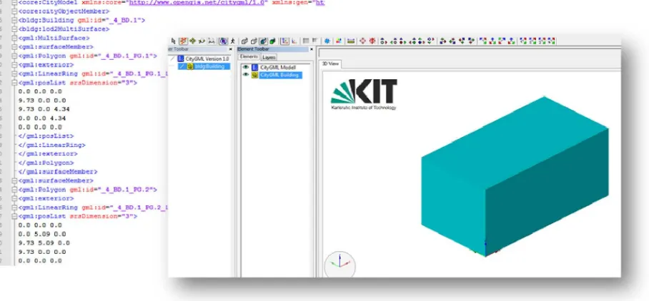
CityGML defines the classes and relations for objects in cities with respect to their geometrical, topological, semantical and ap-pearance properties. This information is stored in a structured XML-based format with different tags for identifications. Fig-ure 3 shows a representation of a single building in CityGML data. CityGML constructs a building with four fac¸ades by having 6 polygonal faces consisting of quadrilaterals defined by the co-ordinates(x, y, z)of their vertices each. The 6 polygonal faces can be identified asgml:Polygontags. Whereby each tag has its own uniquegml:idattribute name identification. For each polyhedron, there is a sub-child tags namedgml:LinearRing
andgml:PosList. Information regarding coordinates are stored ingml:PosListtags in counterclockwise coordinates sequences for faces that are facing outside and clockwise coordinates se-quences for faces that are facing inside. A four sided rectangle is represented by 5 tuples of coordinates(x, y, z). Usually the first and the fifth coordinate sets refer to the same coordinate values in order to create a boundary for the polyhedron. Basi-cally, this sequence is a cycle of coordinates (points). Polyhe-drons that “belong” to a building are grouped in the same set. In the example shown (see Figure 3), the group can be identified as
bldg:Buildingtags.
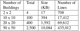
However, CityGML requires 3.12KB of memory / disk storage for the building in Figure refCEDS3 (102 lines of tags and el-ements in XML structure). Table 1 shows the storage size for different numbers of LoD1 objects in CityGML. Retrieving in-formation from CityGML data requires an XML tag list search-ing. The comparison in Table 1 shows a total line of tags for each category for a number of buildings.
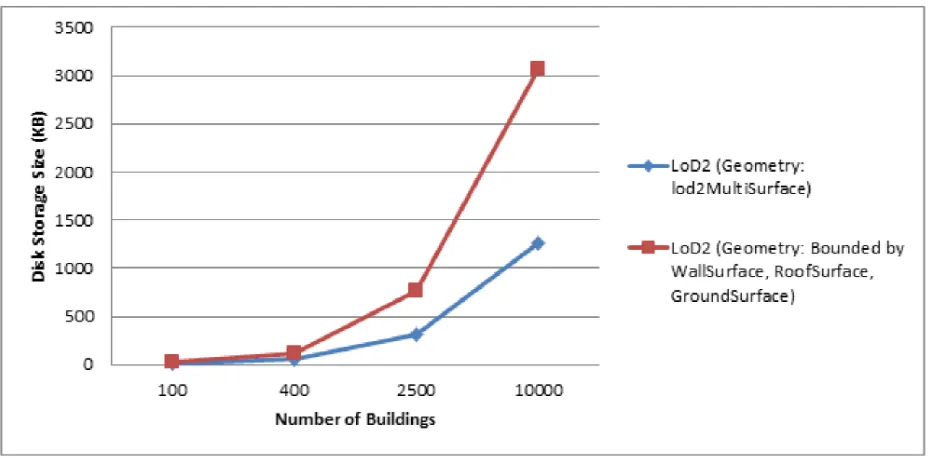
Meanwhile, Figure 4 shows the disk storage comparison of LoD2 objects. Data used as a benchmark test in Figure 4 are down-loadable atwww.citygmlwiki.org. Categorizations were made based on two categories which are LoD2 MultiSurface and LoD2 bounded by WallSurface, RoofSurface and GroundSurface. LoD2 bounded by WallSurface, RoofSurface and GroundSurface is a method of classifying the 3D objects into several parts such as wall, roof or ground surface of a building. This is a common way of describing CityGML data for 3D implementations. Figure 4 shows that the disk storage for LoD2 bounded by WallSurface, RoofSurface and GroundSurface rocketed more than double of LoD2 MultiSurface disk storage size. This graph indicates that it is vital to organize 3D city model data for optimizing 3D spatial queries searches.
Figure 1: LoD2 building illustration: CityGML feature structure as UML instance diagram (taken from (Gr¨oger and Pl¨umer, 2012))
Figure 2: The four levels of detail (LoD) defined in CityGML (taken from (Gr¨oger and Pl¨umer, 2012))
Figure 4: Disk storage comparison between two LoD2 categories
4 SPACE-FILLING CURVES AND HILBERT’S CURVE
A space-filling curve is a continuous function with its domain in-terval[0,1]and its range could be in any topological, uniform or Euclidean space. Space-filling curves allow a proximity prob-lem to be reduced from higher dimensional spaces to a binary search through a one-dimensional space. Such proximity prob-lems usually involve sorting in a one-dimensional space. Many applications can be benefited from space-filling curves, but the most common application of space-filling curves is for storage and retrieval of multidimensional data in a spatial database. A proximity problem for which space-filling curves have been used regularly is the approximate nearest neighbor search or finding closest points from one location. Until now, there are several variants of space-filling curves such as Hilbert’s curve, Dragon Curve, Gosper’s Curve, Moore’s Curve, Z-Order and many more.
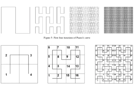
The space-filling curve was discovered by Giuseppe Peano in 1890 and called the Peano’s Curve (Peano, 1890). From his find-ing, a curve must pass through every point on a plane at least once. But, before his finding, in 1878, George Cantor has demon-strated a one-to-one correspondence between the unit interval and the unit square (Thiele and Wos, 2002). In 1879, Netto added that any such mapping could not be continuous. In 1891, David Hilbert discovered the Hilbert Curve structure, which is a simpler variant of the same idea of Peano’s space-filling curve (Kevin, 2008). The Hilbert Curve subdivides squares into four smaller squares instead of Peano’s nine smaller squares. Figure 5 shows four iterations of Peano’s Curve.
When David Hilbert discovered a variation of Peano’s Curve, he divided each side of unit square into two parts equally. This yields the square into four smaller squares. From the divided squares, each of them is divided into another four smaller squares, and so on. For each part of this division, a curve will traverse all the squares. The Hilbert’s Curve normally starts at the lower left division and ends at the lower right division. According to its movement and process, the Hilbert’s curve could be expressed in base 2.
The Hilbert space-filling curve could be described as an under-lying grid, aN×N array of cells whereN = 2n
. Hilbert’s
enumeration of the squares is shown in Figure 6 forn= 1,2,3. Note that the first square is always at the lower left corner and the last square is always in the lower right corner.
From the divided square, we assume that theN×Ncells coordi-nates start at(0,0)in the lower left corner. From the assumptions, Hilbert’s curve has corners at integers ranging from0to2n
−1 in bothxandyand we take a positive direction along the curve from(x, y) = (0,0)to(x, y) = (2n
−1,0).
4.1 Mapping Points Using Hilbert’s curve
Figure 7 shows a set of points that will be used to demonstrate the 2D Hilbert’s space-filling curve.
Figure 7: Scattered points (Kevin, 2008)
Figure 5: First four iterations of Peano’s curve
Figure 6: The first three stages in generating Hilbert’s curve
• Each unit interval and unit square is divided into four inter-vals as shown in Figure 8. Every unit interval is assigned to one square. Figure 8 (a-c) shows the first three steps of this construction. At the limit (when the number of elements goes towards infinity), this produces a subjective, continu-ous map from the unit interval to the unit square.
• Figure 8 (d) shows the resulting order of scattered points in Figure 7. Since the Hilbert’s curve starts in the lower left corner and ends in the lower right corner, the last edge of the round-trip (shown in Figure 8 (d) as dashed lines) from the last corner back to the first corner is much longer than its Euclidean distance.
Figure 9: Possible approach of 3D Hilbert order where n = 2 (Haverkort and Walderveen, 2008)
In this research, we adopt space-filling curves for the ordering in 3D city models. In mathematical analysis, a space-filling curve is a curve whose range contains the entire 2-dimensional unit square (or more generally a n-dimensional hypercube). This space-filling curve visits every point in a square grid with a size ofn2. Space-filling curves in this research were used to compress the three-dimensional models to a one-three-dimensional ordering. Based on previous research in implementing 3D Hilbert’s curve for spatial
structures, there are 1536 diverse methods of 3D Hilbert’s curve implementation (Haverkort and Walderveen, 2008). Meanwhile, Figure 9 shows the 3D Hilbert’s curve implemented in this re-search with the same size2n
and the rationalization of the test data based on simple 3D city buildings. We believe that this 3D Hilbert curve will benefit transportation and air pollution applica-tions, where most of the important spatial adjacencies happen in a single horizontal layer. Results from the implementation of 3D Hilbert’s curve for 3D city model will be discussed in the next section while showing the advantages of smaller data retrieval time and processing.
Figure 10: 3D Hilbert Order
5 ANALYSIS AND RESULTS
sac-Figure 8: Hilbert’s curve and Order (taken from (Kevin, 2008))
rifice the computational performance instead of using it for more intricate procedures.
Since indexing improves the data retrieval capabilities, two types of search analyses were performed. Those analyses are single ject search and nearest object from target search. The single ob-ject search usually is implemented in cases where the user wants to identify a single object from the 3D city model data. For an example, search based on building names or ID. Meanwhile the nearest object from target search is meant for queries like find-ing the adjacent buildfind-ings or pinpointfind-ing nearest facilities from the current location. In comparison, two analyses were prepared for different data sets of buildings (10, 50, 100, 200, 400, 600, 800 and 1000 buildings). Data retrieval times were measured in milliseconds and it was tested in a system using a single Intel Core i7 running at 2.2GHz with 8GB of Random Access Mem-ory (RAM).
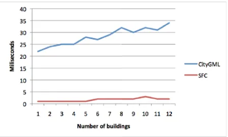
The graph shown in Figure 11 shows two types of 3D spatial data sets used in the single object search: CityGML data and 3D spa-tial data with space-filling curve implementation. The ordering for space-filling curve is based on our 3D Hilbert’s curve imple-mentation. Eight data sets were prepared for each type respec-tively. From the figure shown, it indicates that for single object search, there is not much difference in time measured between both types of sets. This is due to the single object search routine is based on line tags list searching. Times measured in Figure 11 included times for displaying tags that had been traversed before getting to the target object.
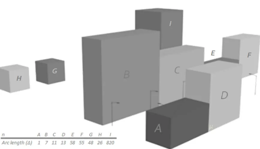
On the other hand, the advantage of space-filling curve operations can be seen in the consistency between neighboring pixels. In this case, the adjacencies between spatial objects were conserved and retrievable. The example shown in Figure 12 identifies ob-jects (buildings) that are located “closed to” the building of inter-est. Since the Hilbert’s curve is organized into a one-dimensional structure, finding the nearest building to a specific building (n) is done by first finding the nearest arc length tonand then checking whether this corresponds indeed to the closest neighbor. Indeed, the ordering induced by the difference (∆) of arc length does not correspond to the ordering of the distance between the projection of the object onto the Hilbert’s curve and buildingn.
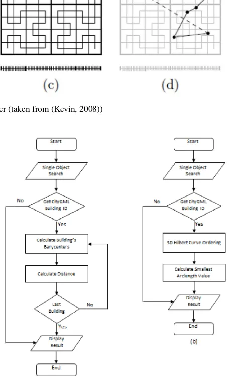
Another experiment conducted in this research is to test the per-formance in data retrieval time for finding the nearest building from the target building. Figure 13 illustrates flowcharts in both implementations for comparison assessment. For this experiment, displaying the traversed tags is excluded and only finding the nearest building is the sole objective. Table 2 and Figure 14 show
Figure 13: Flowcharts for finding the nearest building for CityGML data (a) and with 3D Hilbert’s curve implementation (b)
the running times for queries performed and measured for finding the nearest building to the target building.
Figure 11: Data retrieval time for single object from target search
Figure 14: Data retrieval time for nearest object from target search
Target Nearest CityGML space-filling Elapsed Building Building (ms) curve (%)
ID ID (ms)
Table 2: Data retrieval time for nearest object from target search
6 CONCLUSIONS
In spatial applications, to load the entire 3D city model into a viewer will consume computational processing time, and in some applications it might not be necessary at all. Researchers are facing problems in finding which visualization technique is best suited for displaying 3D city data (M´etral, C. et al., 2012). As an example, in an indoor environment, a room is bounded by doors, windows, walls, corridors, and floors. To make the whole 3D city model reachable at one single processing time is not feasible nor necessary. Practically, by using space-filling curves imple-mentation, knowing which objects are within view of sight will improve the visualization and optimize the memory. Meanwhile, for mobile applications, displaying all 3D objects in a single dis-play consumes a lot of processing-memory allocation and will decrease the device performance. By knowing which 3D objects have their projection on the 3D Hilbert curve within some arc-length from the current location’s projection would be a great idea
for mobile display.
We have proposed a new 3D Hilbert’s curve as a space-filling curve technique, that could be seen as an alternative to CityGML for optimizing query performance. We also demonstrated the query performance comparison of 3D building data set with and without 3D Hilbert’s curve implementation. From the test, we could see that the implementation of space-filling curve method shows advantages in fast acquiring and information retrieval for 3D city model data. The advantages of space-filling curve in preserving neighboring information can be exploited for 3D city model application. However, further studies need to be conducted. This research only focused on buildings as the 3D city object. Since 3D city objects are becoming more sophisticated, other cat-egories of city objects and their relationships are needed. Exper-iments on street furniture and any other objects included in the CityGML standard should be implemented.
7 ACKNOWLEDGEMENTS
Major funding for this research was provided by the Ministry of Higher Education Malaysia and partial funding was provided by the Land Surveyors Board of Malaysia. This work was done while the second author was Visiting Full Professor at the 3D GIS Research Group, Faculty of Geoinformation and Real Estate, Universiti Teknologi Malaysia, for which he is very thankful.
REFERENCES
Behley, J. and Steinhage, V., 2009. Generation of 3D City Models Using Domain-Specific Information Fusion. In: Fritz, M and Schiele, B and Piater, JH (ed.), Computer Vision Proceedings, Lecture Notes in Computer Science, Vol. 5815, pp. 164–173.
Dash, J., Steinle, E., Singh, R. and Bhr, H., 2004. Automatic building extraction from laser scanning data: an input tool for disaster management. Advances in Space Research 33(3), pp. 317 – 322.
Freitas, M., Sousa, A. and Coelho, A., 2010. A visualization paradigm for 3d map-based mobile services. Communications in Computer and Information Science 68 CCIS, pp. 89–103.
Gr¨oger, G. and Pl¨umer, L., 2012. Citygml - interoperable se-mantic 3d city models.{ISPRS}Journal of Photogrammetry and Remote Sensing 71(0), pp. 12 – 33.
Haverkort, H. and Walderveen, F. V., 2008. Space-filling curves for spatial data structures.
Jazayeri, I., 2012. University of Melbourne, chapter Trends in 3D land Information Collection and Management, pp. 81–87.
Jin, B. and Bian, F., 2006. Study on visualization of 3d city model based on grid service. Jisuanji Gongcheng/Computer Engineer-ing 32(4), pp. 217–219+235.
Karlsruhe Institute of Technology, 2013. Ifcexplorer for citygml. http://www.iai.fzk.de/www-extern-kit/index.php?id=1570L=1.
Kevin, B., 2008. Organizing Point Sets. PhD thesis, Freie Uni-versitat Berlin.
Liu, L. and Fang, J., 2009. An accelerated approach to create 3d web cities. In: Geoinformatics, 2009 17th International Confer-ence on, pp. 1–4.
Mao, B., Ban, Y. and Harrie, L., 2011. A multiple representa-tion data structure for dynamic visualisarepresenta-tion of generalised 3d city models. {ISPRS}Journal of Photogrammetry and Remote Sensing 66(2), pp. 198 – 208.
M´etral, C., Ghoula, N. and Falquet, G., 2012. An ontology of 3d visualization techniques for enriched 3d city models. In: Usage, Usability, and Utility of 3D City Models, p. 02005.
Nichol, J. E., Wong, M. S. and Wang, J., 2010. A 3d aerosol and visibility information system for urban areas using remote sens-ing and{GIS}. Atmospheric Environment 44(2122), pp. 2501 – 2506.
Over, M., Schilling, A., Neubauer, S. and Zipf, A., 2010. Gener-ating web-based 3d city models from openstreetmap: The current situation in germany. Computers, Environment and Urban Sys-tems 34(6), pp. 496 – 507.
Peano, G., 1890. Sur une courbe, qui remplit toute une aire plane. Mathematische Annalen 36(1), pp. 157–160.
Thiele, R. and Wos, L., 2002. Hilbert’s twenty-fourth problem. Journal of Automated Reasoning 29(1), pp. 67–89.
Tomaszewski, B., 2011. Situation awareness and virtual globes: Applications for disaster management. Computers Geosciences 37(1), pp. 86 – 92.
van Lammeren, R., Houtkamp, J., Colijn, S., Hilferink, M. and Bouwman, A., 2010. Affective appraisal of 3d land use visu-alization. Computers, Environment and Urban Systems 34(6), pp. 465 – 475.
Zhang, J. and Shen, T., 2008. Research on construction of large-scale 3d city models based on skyline prototype system. Vol. 7143.