A PRELIMINARY STUDY ON MECHANISM OF LAI INVERSION SATURATION
Jing Zhaoa,b, Jing Lia, Qinhuo Liua, Le Yanga
a
State Key Laboratory of Remote Sensing Science, Institute of Remote Sensing Applications, Chinese Academy of
Sciences, 100101, Beijing, China;
b
Graduate University of Chinese Academy of Sciences, Beijing 100039, China
Commission I/2
KEY WORDS: Leaf area index, saturation, vegetation index, PROSAIL, MIMICS
ABSTRACT:
Many parameters, such as albedo, vegetation index and leaf area index (LAI) inversed from satellite images, often get saturated when the surface vegetation cover reaches a certain high level. In order to analyze the saturation phenomena in parameter inversion, we analyze the changing of canopy reflectance and backscattering with increasing of LAI through PROSAIL and MIMICS model respectively. The results show that the canopy reflectances get saturated when LAI exceed 3, and the crown backscatters have strong relationship with biomass, which changes at various incident angles and frequencies. When LAI>3, the reflectance variations between red band and near-infrared band were no longer obvious with the vegetation growing, which directly leaded to the vegetation indices and LAI saturation. This paper is an exploratory research about the LAI saturation, and the reducing saturation methods still need further studies.
1. INTRODUCTION
Leaf area index (LAI) defined as half the total foliage area per unit ground surface area (Chen, 1992), was a key parameter in physical and biological processes of plant canopies. Vegetation index is another indicator of vegetation greenness. Most vegetation indices based on the contrast between the maximum absorption in the red due to chlorophyll pigments and the maximum reflection in the infrared caused by leaf cellular structure. Because of the close correlation between vegetation index and LAI, their relationships always use to estimate LAI. The disadvantage of this method is that the relationship between these two variables tends to saturation at higher LAI.
Many researchers have pointed out that the Normalized Difference Vegetation Index (NDVI) got saturated at LAI values from 1.5 to 3.5 for different types of vegetation e.g. forest, cereal and broadleaf crops (Ludeke, 1991; Myneni, 1997; Anderson, 2004; Gitelson, 2004; Haboudane, 2004a; González-Dugo, 2006; Le Maire, 2006; Wang, 2007; Wu, 2008; Herrmann, 2010; Ferrara, 2010). Other vegetation indices (e.g. Modified Simple Ratio (MSR), Ratio vegetation indices (RVI), Normalized Difference Water Index (NDWI), Optimized Soil Adjusted Vegetation Index (OSAVI), Modified Soil-Adjusted Vegetation Index (MSAVI), Modified Triangular Vegetation Index (MTVI), Renormalized Difference Vegetation Index (RDVI), Modified Chlorophyll Absorption Ratio Index (MCARI) and Soil and Atmospherically Resistant Vegetation Index (SARVI)) were generally saturation at LAI values from 3 to 6 (Gitelson, 2004; Wu, 2008; Xue, 2004; Haboudane, 2004b).
In fact, whether using physical models or empirical methods, the relationships between inversed LAI and canopy reflectance and spectral indices would became saturated in high density of vegetation places. Weiss demonstrated that the neural network method couldn’t discriminate LAI from 4 to 8 due to reflectance saturation (Weiss, 1999). Using leaf-level PROSPECT model and canopy-level SAILH model, Haboudane simulated the MTVI2 and MSAVI2 indices on a series of leaf and canopy parameters. These two indices and LAI had strong linear trends without clear saturation at high
LAI levels (up to 6) (Haboudane, 2004b). Nowadays, the widely used LAI products e.g. MODIS LAI products which based on three-dimensional radiative transfer algorithm (Yang, 2006) and CYCLOPES LAI products which employed neural networks based on PROSAIL radiative transfer model, LAI values always saturated between 4 and 5 (Baret, 2007).
This paper is an exploratory research about the LAI saturation. Based on in-situ measurements in Huailai and simulation results from the optical and microwave models, we try to analyze the LAI saturation factors. Several methods could be reducing the vegetation saturation phenomena, but they still need further studies.
2. SIMULATION AND EXPERIMENT ANALYSIS
In 1953, Monsi and Saeki had pointed out that the relationship between extinction coefficient and leaf area was approximately exponential, and will reach asymptotic at certain conditions. In order to understand the canopy attenuation effects, we carried out an experiment in August 2011, in Huailai, Hebei Province, China. Besides, we apply the PROSPECT and SAIL model to simulate canopy reflectance and MIMICS microwave model to simulate backscatter of canopy at various LAI values, and then discuss the mechanism of vegetation saturation. Results show that the optical model simulations get saturated at moderate LAI value (2~3), and the microwave model results affected by some factors, the trends of results need detailed descriptions.
2.1 Optical model simulation
PROSPECT (Jacquemoud, 1990) is a radiative transfer model based on Allen's generalized plate model that represents the optical properties of plant leaves from 400nm to 2500nm. SAIL model (Verhoef, 1984) considered the arbitrary leaf inclination angle and random leaf azimuth distribution. Kussk considered the hotspot effect into SAIL model and promoted the SAILH model. Now, the combination of PROSPECT and SAIL i.e. PROSAIL model is the most widely used canopy reflectance model (Jacquemoud, 1993).
We use the PROSPECT and SAILH model to simulate canopy reflectance on different LAI values. There are four variables in the PROSECT model and twelve variables in the SAILH model. The mainly input parameters of the PROSAILH model involved in this paper are summarized in table 1. The solar zenith angle θi and viewing zenith angle θv represent the geometry conditions. The leaf biochemical properties and the canopy structure parameters are obtained from LOPEX'93 project measurements.
Parameters Symbol Values
Geometry parameters
Solar zenith angle θi 30
Viewing zenith angle θv 0
Leaf biochemical properties
Chlorophyll a b concentration Cab 52.74 Carotenoids concentration Car 10 Leaf protein content Cm 0.003662 Leaf water content Cw 0.0131 Leaf structure parameter N 1.518 Canopy structure parameters
Leaf area index LAI 0.1-8
Leaf angle distribution LAD 50 diffuse/direct radiation skyl 0.7
hot spot hspot 0.2
Table 1. Input parameters of PROSPECT and SAILH model.
The reflectance estimates in four visible and near-infrared bands, including blue band (445 nm), green band (550 nm), red band (670 nm), and near-infrared band (800 nm). Figure 1 shows that the reflectance in the visible regions exhibit a nearly flat response once the LAI exceeds 3, while the near-infrared reflectance continue to respond significantly even at higher LAI values (up to 6). Therefore, among the four visible and near-infrared bands, the near-near-infrared band is considered as the most sensitive band of LAI.
Figure 1. The relationship between reflectance at four visible and near-infrared bands and LAI
2.2 Microwave model simulation
Unlike optical radiative transfer theory, the microwave sensors detect the backscatters of object. The backscatter characteristics of different objects or components have significant discrepancy. The MIMICS model is chosen for simulating the forest canopy backscatter in the study.
Michigan Microwave Canopy Scattering model i.e. MIMICS (Fawwaz, 1990) model is a radiative transfer model for radar backscattering from forest canopies. The model depicts both like and cross polarized scattering in the canopy at microwave frequency ranges. LAI is not an inner parameter in MIMICS model, but it has connection with leaf number density (Nleaf), crown layer height (H) and mean leaf diameter (dleaf) parameters of MIMICS model. The expression is given by:
2
( / 2) leaf leaf
LAIN H d (1)
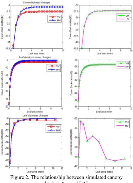
In MIMICS model, the angle of measurement data is valued 30 (degree) and C band frequency of operation data is 5.3 (GHz), the leaf number density is valued equally intervals between 10 and 1500 (leaves per cubic meter), the crown layer height is set from 0.2 to 4 meters, and the mean leaf diameter is valued from 1 to 9 centimetres. In this part of analysis, we change the single factor values while others remain the same.
The relationship between canopy backscatter simulations and LAI is shown in figure 2. For the like polarization (including HH and VV polarization), the crown backscatter coefficient changes have the same trend. The backscatter increase with LAI incremental until LAI up to 3, and then get saturated. The cross polarized scattering coefficient indicate the crown characters in microwave. The cross polarized backscatter increase with LAI incremental at moderate LAI (3~4) and then reach saturation. Among the three parameters, leaf diameter is the key factor influencing the crown backscatter.
Figure 2. The relationship between simulated canopy backscatter and LAI
The factors influencing microwave backscatters are complicated. The simulations will differ from different vegetation structure parameters, incident angles and frequencies. Besides, in the microwave model, the backscatter coefficient of crown includes two components (the leaves and branches), which means the simulations have strong relationship with biomass (figure 2). In fact, the LAI changes depend on leaf number density, crown layer height and mean leaf diameter, and the three factors did not independent with each other.
2.3 Experiment results
The experiment site is located in Huailai (115.78°E, 40.35°N), Heibei province, China. The experiment aims to measure the International Archives of the Photogrammetry, Remote Sensing and Spatial Information Sciences, Volume XXXIX-B1, 2012
light transmissivity and LAI of the corn at different heights (0m, 0.5m, 1m, 1.5m and 2m). The spectral reflectance data over the region from 400nm to 2500nm were acquired with the ASD spectroradiometer. The white Spectralon reference panel was used to calibrate the spectroradiometer spectral radiance and measurement the light transmittance from canopy crown. Corn LAI values measured using the Plant Canopy Analyzer LAI-2000 before 10 o’clock in the morning.
The experiment results show that, the canopy transmissivity reduced and LAI increased with height increasing (figure 3). On the top of canopy at 2m, where leaves distributed sparseness and all leaves under adequate sunlight conditions, we measured the maximum transmissivity and the minimum LAI here. In the middle of canopy, where leaves grow flourish and intercept more sunlight, the transmissivity reduced drastically at height from 1 to 2m. From middle of canopy to the ground (0~1m), only little sunlight could transmit the whole canopy. The reason leading to figure 3’s result is that the corn leaves mainly growth in the middle of canopy; therefore the transmissivity and LAI reached the threshold value at this layer.
Figure 3. Experiment of measuring corn canopy transmissivity and LAI
3. SATURATION ANALYSIS
As mentioned above, many researchers had pointed out the saturated phenomena between reflectance or vegetation indices and LAI. Two questions will arise: the one is what saturation; the other is how to define the vegetation saturation. The following parts will answer these questions.
3.1 Definition of saturation
Saturation refers to the values reached the highest limit among ranges in literal. However, for the non-linearly relationships, the curves always get asymptotic at certain values instead of reach the highest limit value. Therefore, saturation defines as the phenomenon of the external variables changes became stable at certain values of the independent variables. The saturation point refers to the specific values of independent variable when the external variables changes firstly reach asymptote.
3.2 Reasons for NDVI saturation
Under conditions of high aboveground biomass and high vegetation coverage, vegetation indices occurs different degrees of saturation. While the forest growth much denser, vegetation indices were no longer increased with biomass accumulation. Let’s take the NDVI for example, analyze the reasons why NDVI values reached saturation.
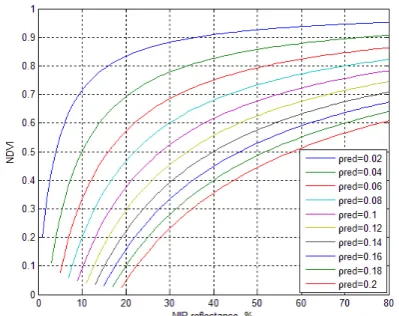
From the definition of vegetation index, both the red and near-infrared reflectance will determine the values of NDVI. In the red wavelength regions, the chlorophyll has a strong absorbance peak, and the maximal absorbance occurs between 660nm and 680nm. When the chlorophyll-a concentration exceeds a certain threshold, the sensitivity of chlorophyll reduced drastically in the red region (Wu, 2008; Yang, 2008). In the near-infrared region, the reflection was cause by leaf cellular structure. In the stage of LAI from 0 to 2, the near-infrared reflectance increased rapidly with LAI raising. Even though the vegetation reached full cover, due to the strong scattering in near-infrared region, the reflectance still enhanced slowly with LAI increasing (Tang, 2003). The NDVI sensitivity for the reflectance was dependent upon the ρNIR/ρred ratio, it’s decreasing with an raising of the ratio (Gitelson, 2004). The simulation results and reference documentations have the identical conclusion (Figure 1). When the red reflectance is smaller than 8%, NDVI was sensitive to changes in near-infrared reflectance below 25-30%, and little sensitivity to changes in near-infrared reflectance above 30%. When the red reflectance is greater than 10%, the relationships between NDVI and near-infrared reflectance presented linear trend (figure 4).
Figure 4. NDVI and NIR reflectance plot under various Red reflectance conditions
In conclusion, on the same vegetation coverage, the difference between red and near-infrared reflectance increased slowly along with leaf area index increasing. Meanwhile, the sum of two bands also increased with leaf area index increasing. Then the NDVI approaches saturation when the increment of the difference or the sum of red and near-infrared reflectance close to equality.
3.3 Reasons for LAI saturation
LAI saturation depends on the difference of canopy reflectance changes with LAI increasing. The mainly problems of the LAI got saturated with vegetation indices depend on leaf biophysical parameters differences (e.g. pigments, internal leaf structure, leaf orientation), tree crown structures differences (e.g. clumping and woody material contribution to total reflectance, tree height heterogeneity and the size and number of tree gaps) and discrepancies in understory contributions and background materials (e.g. understory type, soil properties and soil moisture content) (Iiames, 2008). In fact, the chlorophyll content and the green leaves amount were two major factors determining LAI values (Haboudane, 2004a).
In addition, LAI saturation is strongly related to the species of biomes (Zhang, 2000), spatial variations in environmental stress (Brantley, 2011) and view directions (Asrar, 1992). Grasses and shrubs have nearly no saturation, while broadleaf forests have the highest frequencies of getting saturated (Zhang, 2000). The magnitude of canopy reflection along oblique view directions saturates at a lower value of canopy leaf area index than in near-nadir directions (Asrar, 1992).
The saturation of LAI and NDVI relationship was related to different vegetation growing seasons (Wang, 2005). There were strong linear relationships between LAI and NDVI during the leaf production period and leaf senescence period. On the contrary, there was no clear relationship between NDVI and LAI after leaf monopoly period and harvest period.
In summary, the reasons of LAI got saturated were much more complicated than NDVI.
3.4 Reduce saturation methods
The practical way of decreasing the saturation in NDVI and LAI relationship is to develop new vegetation indices. For example, Gitelson proposed a simple modification of the NDVI named the Wide Dynamic Range Vegetation Index (WDRVI) (Gitelson, 2004). He use the weighting coefficient α to adjusting the linearizing the relationship for typical crops. The sensitivity of the WDRVI to moderate-to-high LAI (from 2 to 6) was at least three times greater than that of the NDVI (Gitelson, 2004). In addition, the reflectance of red and blue band stopped changes when LAI increased up to 3 or 4, but the green reflectance didn’t obviously reach an asymptote even LAI was beyond 5 or 6 (Wang, 2007). Combined with blue and green bands, Wang brought up a new vegetation index named green-blue NDVI (GBNDVI). The results showed that GBNDVI values didn’t obviously reach a saturation level when LAI exceed 4.
An effective way to improving the precision of LAI inversion is combine the mutli-angle data or microwave remote sensing data. Zhang had proposed that LAI saturation frequency decreased with an increased in the number of view angles (Zhang, 2000). Multi-sensor data may help to solve the saturated problem, for example microwave technology could acquire information of vegetation when optical techniques fail to do. Clevers combined a simple reflectance and backscatter model to estimating LAI. Results show that radar recordings at L-band HH polarization or C-band VV polarization gave a slight improvement of the crop monitoring and yield estimation comparing with the optical data alone (Clevers, 1996).
4. CONCLUSION
This paper aims to analyze the reasons causing LAI and vegetation indices saturated. Some researches had demonstrated that the spectral vegetation indices especially NDVI reached a saturation level when LAI exceeds 3. In this paper, we simulate canopy reflectance and backscatter at various LAI based on PROSAILH and MIMICS model respectively. From above analyses, we conclude that canopy reflectance get saturated when LAI exceed 3, and the backscatter changes at various incident angles and frequencies.
The reasons of vegetation indices get saturated mainly lie in the reflectance variations of red and near-infrared band decreased
in the same level. With the plants growth, when the chlorophyll-a concentration exceeds a certain range, the red light was no longer sensitive to it and reached saturation. In the near-infrared, the leaves reflectance increased rapidly with leaf area increasing. When the vegetation achieved full coverage, the reflectance changes in near-infrared were slow down. Therefore, the reflectance variations of the two bands with the vegetation growth were not obvious, which directly leaded to vegetation indices and LAI saturation occurs. Besides, the different characters of biomes, sensor geometries and environment conditions might affect canopy reflectance and contribute to LAI inversions saturation.
5. ACKNOWLEDGEMENTS
This work was supported by the national 863 key Project (No. 2009AA122102, 2012AA12A304), and the National Natural Science Foundation of China (No. 40730525). We thank Junhua Bai, Chuanfu Xia and Xin Long for their contribution to the field measurements.
6. REFERENCE
[1] Chen, J. M. and T. A. Black, 1992. Defining leaf area index for non‐flat leaves. Plant, Cell & Environment, 15(4), pp.421-429.
[2] Ludeke, M., A. Janecek, et al., 1991. Modelling the seasonal CO2 uptake by land vegetation using the global vegetation index. Tellus B, 43(2), pp.188-196.
[3] Myneni, R. B., R. Ramakrishna, et al., 1997. Estimation of global leaf area index and absorbed PAR using radiative transfer models. Geoscience and Remote Sensing, IEEE Transactions on, 35(6), pp.1380-1393.
[4] Anderson, M., C. Neale, et al., 2004. Upscaling ground observations of vegetation water content, canopy height, and leaf area index during SMEX02 using aircraft and Landsat imagery. Remote Sensing of Environment, 92(4), pp.447-464. [5] Gitelson, A. A., 2004. Wide dynamic range vegetation index for remote quantification of biophysical characteristics of vegetation. Journal of Plant Physiology, 161(2), pp.165-173. [6] Haboudane, D., J. Miller, et al., 2004a. Estimation of leaf area index using ground spectral measurements over agriculture crops: Prediction capability assessment of optical indices. In, ××th ISPRS congress:"Geo-Imagery Bridging Continents", Commission VII, WG VII/1, Citeseerpp. p.6.
[7] González-Dugo, M. and L. Mateos, 2006. Spectral Vegetation Indices For Estimating Cotton And Sugarbeet Evapotranspiration. Earth Observation for vegetation monitoring and water management, AIP Conference Proceedings, Naples, American Inst. Physics,852pp. 115-123. [8] Le Maire, G., C. François, et al., 2006. Forest leaf area index determination: A multiyear satellite-independent method based on within-stand normalized difference vegetation index spatial variability. Journal of Geophysical Research, 111(G2), pp.G02027.
[9] Wang, F. M., J. F. Huang, et al., 2007. New vegetation index and its application in estimating leaf area index of rice. Rice Science, 14(3), pp.195-203.
[10] Wu, C. Y., Z. Niu, et al., 2008. Estimating chlorophyll content from hyperspectral vegetation indices: Modeling and validation. Agricultural and Forest Meteorology, 148(8-9), pp.1230-1241.
[11] Herrmann, I., A. Pimstein, et al., 2010. Assessment of Leaf Area Index by the Red-edge Inflection Point Derived from International Archives of the Photogrammetry, Remote Sensing and Spatial Information Sciences, Volume XXXIX-B1, 2012
VENμS Bands. Proc. of the ESA Hyperspectral Workshop, Frascati (Italy),pp.1-7.
[12] Ferrara, R. M., C. Fiorentino, et al., 2010. Comparison of Different Ground-Based NDVI Measurement Methodologies to Evaluate Crop Biophysical Properties. Italian Journal of Agronomy, 5(2), pp.145-154.
[13] Xue, L., W. Cao, et al., 2004. Relationship between spectral vegetation indices and LAI in rice. Acta Phytoecologica Sinica, 28(1), pp.47-52.
[14] Haboudane, D., J. R. Miller, et al., 2004b. Hyperspectral vegetation indices and novel algorithms for predicting green LAI of crop canopies: Modeling and validation in the context of precision agriculture. Remote Sensing of Environment, 90(3), pp.337-352.
[15] Weiss, M. and F. Baret, 1999. Evaluation of canopy biophysical variable retrieval performances from the accumulation of large swath satellite data. Remote Sensing of Environment, 70(3), pp.293-306.
[16] Yang, W., B. Tan, et al., 2006. MODIS leaf area index products: From validation to algorithm improvement. Geoscience and Remote Sensing, IEEE Transactions on, 44(7), pp.1885-1898.
[17] Baret, F., O. Hagolle, et al., 2007. LAI, fAPAR and fCover CYCLOPES global products derived from VEGETATION:: Part 1: Principles of the algorithm. Remote Sensing of Environment, 110(3), pp.275-286.
[18] Jacquemoud, S. and F. Baret, 1990. PROSPECT: A model of leaf optical properties spectra. Remote Sensing of Environment, 34(2), pp.75-91.
[19] Verhoef, W., 1984. Light scattering by leaf layers with application to canopy reflectance modeling: the SAIL model. Remote Sensing of Environment, 16(2), pp.125-141.
[20] Jacquemoud, S., 1993. Inversion of the PROSPECT+ SAIL canopy reflectance model from AVIRIS equivalent spectra: theoretical study. Remote Sensing of Environment, 44(2-3), pp.281-292.
[21] Fawwaz, T. U., K. Sarabandi, et al., 1990. Michigan microwave canopy scattering model. International Journal of Remote Sensing, 11(7), pp.1223-1253.
[22] Yang, J., N. Guo, et al., 2008. Ananlyses on MODIS-NDVI Index Saturation in Northwest China. Plateau meteorology, 27(4), pp.896-903.
[23] Tang, S. H., Q. J. Zhu, et al., 2003. Theoretical basis for its application of the three-band gradient difference vegetation index. Science in China (Series D), 33(11), pp.1094-1102. [24] Iiames, J., R. Congalton, et al., 2008. Leaf Area Index (LAI) Change Detection Analysis on Loblolly Pine (Pinus taeda) Following Complete Understory Removal. Photogrammetric Engineering and Remote Sensing, 74(11), pp.1389-1400. [25] Zhang, Y., Y. Tian, et al., 2000. Prototyping of MISR LAI and FPAR algorithm with POLDER data over Africa. Geoscience and Remote Sensing, IEEE Transactions on, 38(5), pp.2402-2418.
[26] Brantley, S. T., J. C. Zinnert, et al., 2011. Application of hyperspectral vegetation indices to detect variations in high leaf area index temperate shrub thicket canopies. Remote Sensing of Environment, 115(2), pp.514-523.
[27] Asrar, G., R. Myneni, et al., 1992. Spatial heterogeneity in vegetation canopies and remote sensing of absorbed photosynthetically active radiation: a modeling study. Remote Sensing of Environment, 41(2-3), pp.85-103.
[28] Wang, Q., S. Adiku, et al., 2005. On the relationship of NDVI with leaf area index in a deciduous forest site. Remote Sensing of Environment, 94(2), pp.244-255.
[29] Clevers, J. and H. Van Leeuwen, 1996. Combined use of optical and microwave remote sensing data for crop growth monitoring. Remote Sensing of Environment, 56(1), pp.42-51. International Archives of the Photogrammetry, Remote Sensing and Spatial Information Sciences, Volume XXXIX-B1, 2012