VARIABLE SELECTION FOR ROAD SEGMENTATION IN AERIAL IMAGES
Sven Warnke, Dimitri Bulatov
Fraunhofer IOSB, Ettlingen, Germany,{name.surname}@iosb.fraunhofer.de
Commission II, WG II/4
KEY WORDS:Classification, Feature Selection, Logistic Regression, Random Forests, Road Extraction
ABSTRACT:
For extraction of road pixels from combined image and elevation data, Wegner et al. (2015) proposed classification of superpixels into road and non-road, after which a refinement of the classification results using minimum cost paths and non-local optimization methods took place. We believed that the variable set used for classification was to a certain extent suboptimal, because many variables were redundant while several features known as useful in Photogrammetry and Remote Sensing are missed. This motivated us to implement a variable selection approach which builds a model for classification using portions of training data and subsets of features, evaluates this model, updates the feature set, and terminates when a stopping criterion is satisfied. The choice of classifier is flexible; however, we tested the approach with Logistic Regression and Random Forests, and taylored the evaluation module to the chosen classifier. To guarantee a fair comparison, we kept the segment-based approach and most of the variables from the related work, but we extended them by additional, mostly higher-level features. Applying these superior features, removing the redundant ones, as well as using more accurately acquired 3D data allowed to keep stable or even to reduce the misclassification error in a challenging dataset.
1. INTRODUCTION
Motivation Extracting roads from remote sensing images is im-portant in a number of different applications, for example traffic management, city planning, road monitoring, GPS navigation and map updating (Wang et al., 2016). However, until now, no fully automated road network detection method is applied in praxis, see Rottensteiner et al. (2013). The reason lies in the difficulty of the classification problem. There are many factors that make road network extraction from remote sensing images challenging. First of all, the dependence on the sensors and resolution cause a variety of problems; moreover, even if same sensors and reso-lutions are used, appearance of roads in remote sensing images can vary wildly. Some reasons are weather and illumination ef-fects and, very importantly, shadows and occlusions caused by high buildings, tree crowns, moving or parking vehicles and tiles of rubbish in developing countries. Because buildings and vehi-cles are indispensable part of urban terrain, road extraction from urban scenes is considered even more difficult than in rural areas (Hu et al., 2014).
Previous work The challenges mentioned above demonstrate that probably any conceivable rule for road pixel extraction from 2D or 3D information has a large number fo counterexamples, both false positive and false negative. One could think about thresholding relative elevations (also knows as normalized Dig-ital Surface Model, nDSM) over the ground; Here, bridges are examples of false negatives and farmlands represent examples of false positives, leaving aside the fact that extraction of ground pixels is not always trivial and widely error-free. Thus, modern approaches use combination of rules that support each other on their way towards a reliable road pixel extraction. Thinkable rules are nDSM, Normal Difference Vegetation Index (NDVI), color information from different color spaces (Wegner et al., 2015), lines detected in images ( ¨Unsalan and Sirmacek, 2012), stripes detected in nDSM for representing street canyons (Hinz, 2004), surface roughness (Hu et al., 2014), spatial signature measure
employed by Jin and Davis (2005), filters, descriptors and tex-tons employed by Montoya-Zegarra et al. (2015); Poullis and You (2010); Wegner et al. (2015), methods based on morphological profiles (Valero et al., 2010) up to the approaches based on Con-volutional Neural Networks (Sherrah, 2016), where the problem is solved by applying very large numbers of features (neurons) and huge amounts of training data.
The variety of rules in this fragment of the seemingly nearly end-less list of ways to extract road pixel confirm the non-triviality of the task. However, one can identify tendencies towards a large number of generic features without explicit semantic meaning. Also, it can be followed that a combined evaluation of features, in particular extracted both in two- and three-dimensional data, is more promising than relying on just one source of information. Accurate, high-resolution 3D information can be extracted by means of a stereo-matching procedure, such as Lemaire (2008).
using the minimum cost paths as higher order cliques. The su-perpixels along the reliable paths are thus encouraged to belong to the road class. The latter two steps of the method can be in-terpreted as post-processing of the classification result obtained by random forests. Obviously, the quality of the final road net-work extraction depends to a great part on the accuracy of this preliminary classification.
Bottleneck: Variable selection Clearly, the main focus of the contribution of Wegner et al. (2015) lay on minimum cost paths. However, we feel that the step of preliminary classification did not receive the attention and care its importance deserves. Espe-cially, in the list of used variables, some of them were quite ob-viously redundant and many useful variables missed. Missed are those higher-level features that allow to combine spectral chan-nels and elevation data and thus may perform better in shadow regions. Redundant features are known to have only marginal detrimental effect on random forests (Genuer et al., 2010), but a dramatic degradation can result for other classifiers, such as lo-gistic regression (Cox, 1958). As a consequence, any method, including the approach of Wegner et al. (2015), could benefit greatly - both with respect to the performance and the comput-ing time - from a careful selection of variables (features).
Methods for automatic variable selection are being applied in ba-sically all machine-learning areas. The dramatically increased amount of data and features – as highlighted in our previous con-siderations – commonly used in modern machine learning due to the growing capabilities of sensors and computers, underlines the importance of automatic feature selection in basically all areas of machine-learning. Additionally, in many applications, expert knowledge is not always available or sufficient to select variables.
Since for a set ofpvariables, the number of possible subsets is 2p
, the problem of variable selection is known to be NP-hard. Hence, no feature selection method that terminates in a reason-able amount of time performs optimally in all situations (Kohavi and John, 1997; Bol´on-Canedo et al., 2015). It is, therefore, not surprising that an immense and ever growing number of different heuristic strategies exist (Bol´on-Canedo et al., 2015; Sta´nczyk and Jain, 2015), so many in fact that it makes choosing one of them difficult since it requires a relatively deep understanding not only of the mechanism of available feature selection meth-ods, but also and in particular, the functionality of the underlying classifier.
Contribution In this work, we adopted from the superpixel-wise classification framework and the features generated from filter banks Wegner et al. (2015); that is, we omitted the post-processing steps in order not to gloss over the raw classification results. However, we extend the variable set of Wegner et al. (2015) by our variables and performed classification with two methods. On the one hand, we applied the random forest clas-sifier, which is a conceptually simple, but powerful tool whose mathematical properties are however not sufficiently explored yet. On the other hand, we employed logistic regression. Although its application is not recommendable if the data cannot be ap-proximately separated into classes by hyper-planes or if variables are strongly correlated, this is actually the reason why we are interested to measure its performance while testing our (some-times highly redundant) variables. Besides, logistic regression is mathematically well understood due to its inclusion into the class of generalized linear models for which properties asymptotic in terms of training data can be proved (Fahrmeir and Kaufmann, 1985; Warnke, 2017).
Inspired by the work of Kohavi and John (1997), we implemented for both classifiers a wrapper framework, which allows computa-tion and evaluacomputa-tion of models with part of the training data and feature subsets. Stepwise forward and backward selection pre-suppose extending or reducing these subsets until some stopping criterion is satisfied. Thus, our main contribution is made up of a simple, yet powerful, method of feature selection with a rather intuitive mechanisms. Furthermore, as all wrappers, it directly links selection to prediction accuracy, a measure whose utility is obvious and which can be tracked back to the visited feature subsets and their evaluation result. For random forest, this is out-of-bag misclassification rate, and for logistic regression, it is the Wald-test. Both are built into their respective models; as a con-sequence, most users will be familiar with them, which keeps the selection process easily understandable.
We applied and evaluated different variable selection methods to road extraction from the Vaihingen dataset (Rottensteiner et al., 2013), an often used benchmark for urban classification from remote sensing. The learning algorithms we used are random forests, as proposed by Wegner et al. (2015), but also logistic re-gression.
Organization The paper is structured as follows. In Sec. 2, we give a description of our wrapper and its application for our classifiers. Note that we will skip the description of these classi-fiers since these are standard, established methods; the interested reader can find their detailed description and critical juxtaposi-tion with respect to feature selecjuxtaposi-tion in Warnke (2017). Next, we discuss in Sec. 3 the relevant features. In Sec. 4, we present our results: Feature sets selected by each classifier and each selection tool as well as their performance. Sec. 5 summarizes the contents of this work and outlines several ideas of future research.
2. WRAPPER METHOD FOR VARIABLE SELECTION There are three general classes of variable selection algorithms. First,filter methodsbasically presuppose assessing each variable’s usefulness through the training data only and discard the less rel-evant variables. Thus, they do not depend on the underlying clas-sifier. Second, methodsembeddedinto the model building pro-cess penalize the models that are too complex, thus allowing to establish which variables best contribute to the model accuracy and which are superfluous. The third category is referred to as
wrapper methods. These are recursive procedures which com-prise: Model inference based on a subset of variables, evaluation of the model using e. g.n-fold cross validation and updating the subset according to the result of the evaluation. The procedure terminates if no better subset was found within the last couple of steps of the search algorithm. Because wrapper methods con-nect variable selection to prediction accuracy of the underlying classifier, they are particularly interesting to the authors.
To summarize, wrapper methods can normally be divided into the following parts, covered in the rest of this section: Starting set,
search algorithm,stopping criterion, andevaluation method. In the following, we will discuss these parts in more detail.
comes from the fact that in the worst case, adding single features requires evaluatingO(p2)models, wherepis the number of fea-tures, which may be very high. To avoid this, depth-first search is simulated. In the second case, known as backward selection, variables are gradually removed from the current set. Because creation of the models containing fewer predictors is less compu-tationally expensive, forward selection is often preferred in praxis due to its greater speed. However, for backward selection, usu-ally, less models have to be instantiated.
As for thestopping criterion, an intuitive way to do this would be stopping as soon as adding a further feature does not improve the accuracy of prediction. However, an extreme example, the well-knownXOR-problem, shows that this strategy is suboptimal and that care should be taken to prevent the algorithm ending up in a local optimum. In the XOR-problem, none of two vari-ables improves the performance, but their combination does. The necessary condition for selecting both relevant variables within a stepwise forward selection algorithm is to let the search terminate if in at least the last two steps no improvement has been achieved. Note that this condition is not sufficient, because one of two fea-tures must make it into model up to this point, in order to reach the second feature in the next iteration. It is, however, unlikely if we assume that any of two features has no merit on its own.
The remaining question of evaluation method can always be solved using then-fold cross-validation. It is considered a very reliable way to estimate prediction accuracy of a model (Kohavi and John, 1997), but it is however expensive sincenmodels have to be fitted. Because of this and because of a rather undesired in-variance of this method with respect to the underlying classifier, we are interested to design a classifier-internal evaluation strat-egy. For classifiers selected for this work, namely logistic regres-sion and random forests, the respecting evaluation methods will be reviewed in both concluding paragraphs of this section.
For logistic regression, it is possible to refer to the so called Wald-statistics, which allows to detect which variables of the current set are redundant; during the backward selection, it can be applied either to the current set of features at each iteration, striving to remove one variable, or to the whole set of features if order to filter out the apparently less useful and redundant features. From the asymptotic properties of logistic regression, it is known that the sought parameter vectorβis normally distributed
ˆ
β∼ Nβ0, F( ˆβ)−1
, (1)
whereβ0 is the expectancy andF the Fisher information de-fined as the inverse covariance matrix of the gradient of the log-likelihood function with respect toβ. Using the approximate normality ofβ, the Wald-test is supposed to test the hypothesis H0 :βq+1 = · · · =βp = 0,for someq,0 ≤ q < p, which
would mean that the variables corresponding to the lastp−q en-tries ofβ, βq+1, ..., βpare not needed for our model. To reject
the hypothesisH0, it can be followed that the Wald-statistics
W = ˜βTF˜β˜ ∼χ2p−q
> χ2p−q(0.95), (2)
whereβ˜= [βq+1, ..., βp]T,F˜is the lower(p−q)×(p−q)
sub-matrix ofF, andχ2is the well-known Chi-squared distribution. Note that (2) holds if at least one of the entries ofβ˜deviates from zero and thus, one of the corresponding variables is needed for our model. Of course, in praxis, the test is often used the other way round. A set of predictors is removed from the model if their Wald-statistic is not significant at a predefined level, opting thus
for simpler models once it couldnotbe shown that all predictors of a more complicated one are needed.
For random forests, instead of costly cross-validation, the easily available out-of-bag prediction measure makes possible a much faster estimation of the model prediction accuracy. For a random forestT, the rate ofOut-of-Bag misclassificationis defined as:
EOOB(T) = #1X#{(x, y)∈X|TOOB(x, y)6=y}. (3)
whereXis the set of training samples(x, y)andxandyare the features and the labels, respectively, while#denotes the cardi-nality of a set. Further,TOOB(x, y)denotes the Out-of-Bag
pre-diction for training sample(x, y), i.e. the class that is predicted by the majority of trees withinT where(x, y)was out-of-bag. There is empirical evidence that the accuracy of the Out-of-Bag misclassification rate is almost the same as if one would apply an additional test-set of the same size (Breiman, 1996).
3. EXTRACTED FEATURES
Since the number of features that could possibly be extracted is seemingly endless, this step is always a compromise. On the one hand, we wish to incorporate all the useful information contained in the image material, since due to our subsequent feature selec-tion, we can accept taking in a lot of irrelevant or redundant vari-ables in order to show the capabilities of variable selection. On the other hand, however, too many useless features can become prohibitively expensive for the wrapper methods with respect to computing time. Nevertheless, we align ourselves to the choice of Wegner et al. (2015), extend it by several new features that are popular in photogrammetry and remote sensing, and wish to demonstrate that even after a careful, knowledge-based extraction of features, automatic variable selection is highly beneficial.
A common approach in computer vision is convolving the image material with a number of different filters and taking the result-ing filter responses as features (Cula and Dana, 2004; Varma and Zisserman, 2005; Winn et al., 2005). The applied filters usually detect edges or smoothen the image. For example, Wegner et al. (2015) applied the filter bank of Winn et al. (2005) to each of the three channels of an image, transferred into the opponent Gaus-sian color space (OGC space) (Geusebroek et al., 2001) as well as the relative elevation value. The mean value and standard de-viation of all these features over all pixels of a segment were then the output of their feature extraction procedure. Hence, in total, there were:
{3×3[Gaussians for every channel]+4×2[Filter kinds for the first channel]+1[rel. elevation]} ×2[mean and standard deviation] = 36variables. It seems that some of these predictors are redundant and that some measures (like NDVI, Normal Veg-etation Differential Index), commonly used in classification for remote sensing applications, are not taken into account. For our work, this was the main motivation.
Geusebroek (2009) claim that the filters of Varma and Zisserman (2005) are better suited for application to images in the OGC space while the filter set of Winn et al. (2005) is designed for the Lab color space.
Moreover, we collected unfiltered channels of the orthophoto and nDSM in order to take into account different filter sizes from the Winn bank of filters, preferred by Wegner et al. (2015). We refer to the total of 56 variables:
{8[filters in MR8 filter bank]×3[channels]+3[unfiltered chan-nels]+1[rel. elevation]} ×2 = 56asWegner-like. Addition-ally, we have 22 more variables. The first 16 of them arise from the fact that we also subject the nDSM to the MR8-based filter-ing (note that as always we store average and standard deviation of every segment), and only image channels. The DSMs stem from a very accurate multi-baseline approach. As a consequence, also the features derived from the DSM (planarity, scattering etc.) are highly discriminative and almost comparable with those ex-tractable from laser point clouds.
The remaining six features use combinations of channels. First, the well-known NDVI (also here, average and standard deviation were taken). Second, stripes computed in the nDSM and in the orthophoto were calculated. These stripes are formed from pairs of nearly parallel straight lines detected in the image. For appli-cation of stripes for detecting man-made structures, we refer to Soergel et al. (2006), from where we also took the technical de-tails for the computation of stripes. Stripes are detected in the nDSM and in the intensity image of the orthophoto, thus yielding four more variables. In the following, we summarize the differ-ences between our variables and those of Wegner et al. (2015).
1. Unfiltered channels,
2. Filter bank: MR8 instead of Winn-filters →Wegner-like features,
3. Application of MR8 filter bank to nDSM,
4. NDVI- and stripes-based features.
Classification For training with a certain training set using a specific feature set, the output model is the set of decision trees in case of random forests classifier and the parameter vectorβˆ for logistic regression. For logistic regression, the probabilityP of a superpixel to belong to the road class is given by the logistic function
P= exp( ˆβ
T
x)
1 + exp( ˆβTx), (4)
wherexis the feature vector. For random forests,P is the per-centage of trees which output it as road class (we utilized 200 trees in our experiments). The local classification result is ob-tained by assigning the superpixels the road class ifP > 0.5 and non-road otherwise. Wegner et al. (2015) usedP for their non-local optimization post-processing step.
For convenience, we summarize below our three-step algorithm:
1. Perform variable selection on a part of the training data which yields a feature subset
2. Induce a model using these features and the complete train-ing data
3. Output the probability of the test data.
4. RESULTS
The considered dataset is the publicly available ISPRS bench-mark Vaihingen (a town in Southern Germany) for urban area object classification, see Rottensteiner et al. (2013), provided by the German Society for Photogrammetry, Remote Sensing and Geoinformation (DGPF), Cramer (2010). In total, there are 16 patches containing the images at a resolution≈0.1m, the cor-responding DSMs, created by the method of Lemaire (2008), as well as the labeled ground truth, created by SIRADEL corpo-ration (www.siradel.com). In the images, the near infrared is present instead of the blue channel. For a better overview, we want to outline in Sec. 4.1 important remarks on data prepara-tion as well as the evaluaprepara-tion criteria while in Sec. 4.2, evaluaprepara-tion results will be presented.
4.1 General remarks on preparation of the data
nDSM extraction and superpixel generation Firstly, since the relative elevatation is clearly a more suitable variable for a learn-ing algorithm than the absolute height, we obtained for every patch the nDSM, . This is done by calculating the ground sur-face using the procedure of Bulatov et al. (2014) and subtract-ing it from the DSM. Secondly, segmentation into superpixels is carried out by means of thecompact superpixelsalgorithm (Vek-sler et al., 2010). This algorithm uses for each superpixel a data term, which prevents it from growing outside of a predefined box, and a smoothness term penalizing the weighted number of pix-els shared by two adjacent superpixpix-els. Since this smoothness penalty is submodular, the alpha-expansion method (run over all superpixels and several iterations) with maximum flow (Boykov et al., 2001) as the core methods allows to obtain a strong local minimum of the resulting function. Next, we proposed a filtering procedure, since some segments are too small and do not contain enough information. They are fused with neighbors. In the seg-mentation we used throughout this work, the average number of pixels in a segment as about440and the number of segments thus was around 10 to 12 thousands which makes the test tractable (not more than several seconds).
Features computation Similarly to Wegner et al. (2015), we extracted the mean and the standard deviation for all features over segments. However, since the near-infrared replaces the blue channel, the transformation into OGC-space, originally designed for true RGB images, is, strictly speaking, invalid. Nevertheless, Wegner et al. (2015) converted the image material, treating them just as though they were RGB images without even a side note. Even though this seems questionable, our experience showed that calculating features from the transformed images achieved better accuracy than those extracted directly from the infrared, red and green values. Because of this, because of a consistent compari-son, and because we are planning toevaluateour features rather than fine-tune them, we decided to retain this strategy.
Evaluation strategy The models we compare in this work use feature sets resulting from:
1. The standard forward selection,
2. the standard backward selection,
3. all variables discussed in Sec. 3,
4. all Wegner-like variables,
1. How many variables each of our classifiers considers as nec-essary,
2. how the reduction of variables changes the prediction accu-racy, in particular, with respect to the full set of variables and to the results of related work,
3. overall performance evaluation
4. finally, which are the trend in variables preferred by logistic regression and random forests.
To answer the first question, we successively used each of the seg-mented patches as test data while the remaining patches served as training data. This means that after variable selection, every of 78 features of Sec. 3 can at most be called 16 times. Thus, we can derive the average size of the feature sets produced by the feature selection methods. Analogously, we can store for all variables the number of patches it was needed in, to give answer to the last question. For the second question, we specified, according to Heipke et al. (1997), the standard measures of classification, such as completeness, correctness and quality. To compute these mea-sures, we assessed, which segments lie in ground truth to more than or less than 50% in the street class to obtaintrueandfalse
segments, respectively. From this as well as thepositivesand neg-ativesof our classification result, the measures of Heipke et al. (1997) are derived using the well-known terms. For more thor-ough performance evaluation, for example, ROC curves, we refer to Warnke (2017), since otherwise we would explode the scope of this work. Thus, a brief reference to two classification exam-ples will be provided to respond to the third question and a few concluding recommendations on the selection of features for both classifiers are given to provide an answer of the fourth question.
4.2 Evaluation
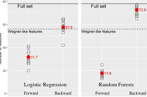
Reducing feature set We start analyzing the overall perfor-mance of the variable selection methods with respect to their abil-ity of variable reduction. In Fig. 1 we see the number of variables remaining after running forward and backward selection for both logistic regression and random forests. It is evident that our goal was successfully achieved since feature sets are always reduced to some extent and significantly in three of the four methods. Es-pecially, forward selection brought a considerable improvement: The average number of remaining variables was below 32 for lo-gistic regression and even below 17 for random forests. How-ever, results tend to lie close to the starting point of the search, i. e. the empty set for forward selection and the full set of predic-tors for backward elimination. It may seem worrying: Since for-ward and backfor-ward methods are supposedly optimizing the same target function and only differ in the way they search through the space of candidate subsets, one should expect more similar re-sults. It seems that the search gets stuck in a local minimum after a relatively short time and that this tendency will aggravate with a higher number of features. It is worth mentioning that with re-spect to the backward selection, the situation is considerably bet-ter for logistic regression: Since logistic regression is more sensi-tive towards redundant variables, discarding them usually causes a noticeable improvement. In the case of random forests, redun-dant variables do not have such a negative impact on a models ac-curacy. Although this is a treasured property of random forests, for a wrapper-type feature selection, however, it becomes cum-bersome, since it leads to premature termination of the search. The mentioned differences between forward and backward selec-tion should be kept in mind when choosing a feature selecselec-tion method. As a rule of thumb, forward selection methods are suit-able for a drastic reduction of the varisuit-able set whereas backward methods focus on prediction accuracy.
Forward Backward Forward Backward
Logistic Regression Random Forests
Figure 1: Cardinalities of the produced feature sets for different patches, indicated by black circles; the average cardinalities are depicted in red.
Performance of reduced sets Another good news is that, dis-carding even a significant amount of variables through variable selection does not affect the performance negatively. On con-trary, as shown in Fig. 2, it becomes clear that the reduced set of features can improve the performance for Logistic Regression, while for Random Forests, it remains approximately equal (for the different sensitivity towards redundant variables as explain-ed above). An important point to note is that the addition of features to the Wegner-like features, increased performance no-ticeably. To provide a direct comparison of our method with the actual results of Wegner et al. (2015), it must be kept in mind that the elevation information was computed by a state-of-the-art method and is of a superior quality to that used in their paper. Moreover, the measures of completeness, correctness, and qual-ity of Heipke et al. (1997) depend highly on the discrimination threshold, which was not provided. Nevertheless, we found dis-crimination thresholds for both of our classification methods (0.5 for random forests and 0.65 for logistic regression) that result in improvements in all three of those values at the same time (see Ta-ble 1). Thus, the usefulness of our modifications to the method of Wegner et al. (2015), even after application of the post-processing steps, is shown.
From Table 1, we also gather that random forests outperformed logistic regression. Another point that speaks for the choice of random forests as a learning algorithm over logistic regression within the procedure of Wegner et al. (2015) is the nature of the produced a-posteriori probabilities: Logistic regression tends to output probabilities close to either zero or one, whereas random forests convey uncertainty better, thus making post-processing steps like the proposed minimum-cost paths more promising.
Method Quality Comp-ness Corr-ness
Wegner’s RFs 0.65 0.77 0.81
Wegner’s paths 0.68 0.81 0.81
Our LR 0.692 0.817 0.819
Our RF 0.722 0.846 0.831
Table 1: Comparison of the pixel-wise classification obtained with the results of Wegner et al. (2015, Table 1).
Wegner-like All Forward Backward Wegner-like All Forward Backward Logistic Regression Random Forests
Figure 2: Resulting (superpixel-wise) average class error of the models trained on the feature sets produced by each variable se-lection method for each learning algorithm. Colored points de-note the performance (percentages of falsely classified superpix-els) of the relevant algorithm for the 16 patches. The colored lines and stars stand for average and median values, respectively.
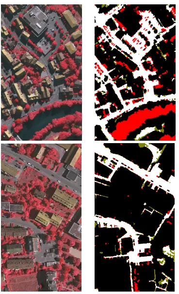
performance of the method quantitatively. However, in Fig. 2, we noticed that the quality of our classification results varies greatly from patch to patch. Hence, our next goal is a qualitative assess-ment of the classification results, for which we refer to Fig. 4, p. 8. It is well-known that road extraction from remote sensing is diffi-cult because of shadows (see Sec. 1), which are the most common reason for misclassification occurence in our results as well. The presence of dark shadows in an urban scene depends on the size of the constructions and trees. Beside, some parts of Vaihingen have many narrow alleys while others are dominated by broad streets. Here is also where the problem of under-segmentation comes into play. Finally, a huge problem for classification are rare types of ground cover. For instance, patch number 26 of the Vaihingen data set is the only one where a river appears. Since its appearance in color, texture, and height resembles impervious surface, it gets misclassified almost completely since the learning algorithms did not see water surface in the training data.
Logistic regression forward Random forests forward
Figure 3: Resulting change in average class error if the models are trained on the variable sets produced for specifically for the other learning algorithm by forward selection. Colored points denote the performance (percentages of falsely classified superpixels) of the relevant algorithm for any of 16 single images. The colored lines and stars represent average and median values, respectively.
Trends of selected features As for variables chosen by both classifiers, Random Forests preferred the (segment-wise) aver-ages to the standard deviations and filtered to the non-filtered features. In forward selection, actually almost all standard de-viations were considered irrelevant, with exception of relative el-evation and filter 1. From the average values, features based on the relative elevation were usually called slightly more often than those based on the three channels of the images. Logistic re-gression almost equally relies on averages values and standard deviations. It takes more variables resulting from the filter bank, especially the 7-th and 8-th filters. Features based on stripes and average of NDVI were selected very often both for logistic
re-gression and for random forests. This supports our expectations about the importance of skillfully combining different channels and developing higher-level features that go beyond the borders of the segments and incorporate context information. For more details, we refer to Warnke (2017).
The feature sets produced by our wrapper-type feature selection methods are specific to the machine learning method for which they were conducted. It can be observed on the right part of Fig. 3 that on average, the set of variables recommended by the forward selection method of logistic regression results in a slightly worse classification accuracy by means of random forests than the fea-ture set customized for this classifiers. On contrary, if we use the set of variables recommended by Random Forests for Logistic Regression as a classifier, the accuracy sinks considerably. The fact that the relevance of different features depends on the ma-chine learning algorithm may appear surprising at the first glance. However, since the mechanisms of these algorithm differ substan-tially, these are also different (aspects of) variables that come into play. This demonstrates, on the one hand, the theoretical strength of wrappers, since they choose variables that are useful for a par-ticular learning algorithm. On the other hands, it helps to em-phasize the importance of easy-to-use variable selection methods that allow every user selecting those variables that are specifically useful for his/her applicationandclassification method.
5. CONCLUSIONS AND OUTLOOK
We investigated the merit of two simple wrapper approaches for variable selection and tested them extensively with two classi-fiers, several dozens of features and an extensive amount of train-ing and test data. From our experiments, we saw that there is a lot of potential for optimizing the classification quality by choosing appropriate variables and performing variable selection both with respect to accuracy and costs. The features we added to those mentioned in Wegner et al. (2015), such as DSM filters, vegeta-tion index and presence of stripes, allowed to achieve a higher accuracy. However, this improved accuracy does not necessarily come at the cost of a bigger feature space. As we have seen, it is possible to reduce the extended feature space, even below the size it had before our features were added, while keeping the accuracy stable or even improving it.
We could see that the relevance of different features depends on the machine learning algorithm. Thus, we demonstrate the the-oretical strength of wrappers, since they choose features that are useful for a particular machine learning algorithm, contrary to filtering methods, which assess suitability of every feature. How-ever, the fundamental differences between the variable sets pro-duced by forward and backward selection should be noted. Con-cerning the choice of classifier, random forests are preferable over logistic regression because they produce a higher classification accuracy. Moreover, as our first experiments showed, they are more suitable for the minimum cost paths employed by Wegner et al. (2015), since they better convey uncertainty which simpli-fies post-processing the results. However, it remains to inspect whether other classifiers like neural networks or support vector machines might lead to even better classification results.
References
Boykov, Y., Veksler, O. and Zabih, R., 2001. Fast approximate energy minimization via graph cuts. IEEE Transactions on pattern analysis and machine intelligence23(11), pp. 1222– 1239.
Breiman, L., 1996. Out-of-bag estimation. Technical report, Cite-seer.
Breiman, L., 2001. Random forests. Machine learning45(1), pp. 5–32.
Bulatov, D., H¨aufel, G., Meidow, J., Pohl, M., Solbrig, P. and Wernerus, P., 2014. Context-based automatic reconstruction and texturing of 3D urban terrain for quick-response tasks.
ISPRS Journal of Photogrammetry and Remote Sensing93, pp. 157–170.
Burghouts, G. J. and Geusebroek, J.-M., 2009. Material-specific adaptation of color invariant features.Pattern Recognition Let-ters30(3), pp. 306–313.
Cox, D. R., 1958. The regression analysis of binary sequences.
Journal of the Royal Statistical Society. Series B (Methodolog-ical)pp. 215–242.
Cramer, M., 2010. The DGPF test on digital aerial camera eval-uation – overview and test design. Photogrammetrie, Fern-erkundung, Geoinformation2, pp. 73–82.
Cula, O. G. and Dana, K. J., 2004. 3d texture recognition us-ing bidirectional feature histograms. International Journal of Computer Vision59(1), pp. 33–60.
Fahrmeir, L. and Kaufmann, H., 1985. Consistency and asymp-totic normality of the maximum likelihood estimator in gener-alized linear models. The Annals of Statistics13(1), pp. 342– 368.
Genuer, R., Poggi, J.-M. and Tuleau-Malot, C., 2010. Variable selection using random forests. Pattern Recognition Letters
31(14), pp. 2225–2236.
Geusebroek, J.-M., Van den Boomgaard, R., Smeulders, A. W. M. and Geerts, H., 2001. Color invariance.IEEE Transactions on Pattern Analysis and Machine Intelligence23(12), pp. 1338– 1350.
Heipke, C., Mayer, H., Wiedemann, C. and Jamet, O., 1997. Evaluation of automatic road extraction. International Archives of Photogrammetry and Remote Sensing32(3 SECT 4W2), pp. 151–160.
Hinz, S., 2004. Automatic road extraction in urban scenes and be-yond. International Archives of Photogrammetry and Remote Sensing35(B3), pp. 349–354.
Hu, X., Li, Y., Shan, J., Zhang, J. and Zhang, Y., 2014. Road centerline extraction in complex urban scenes from lidar data based on multiple features.IEEE Transactions on Geoscience and Remote Sensing52(11), pp. 7448–7456.
Jin, X. and Davis, C. H., 2005. An integrated system for auto-matic road mapping from high-resolution multi-spectral satel-lite imagery by information fusion. Information Fusion6(4), pp. 257–273.
Kohavi, R. and John, G. H., 1997. Wrappers for feature subset selection.Artificial intelligence97(1), pp. 273–324.
Lemaire, C., 2008. Aspects of the dsm production with high res-olution images. International Archives of the Photogramme-try, Remote Sensing and Spatial Information Sciences37(B4), pp. 1143–1146.
Montoya-Zegarra, J. A., Wegner, J.-D., Ladick`y, L. and Schindler, K., 2015. Semantic segmentation of aerial images in urban areas with class-specific higher-order cliques. ISPRS Annals of the Photogrammetry, Remote Sensing and Spatial Information Sciences2(3), pp. 127.
Poullis, C. and You, S., 2010. Delineation and geometric model-ing of road networks. ISPRS Journal of Photogrammetry and Remote Sensing65(2), pp. 165–181.
Rottensteiner, F., Sohn, G., Gerke, M. and Wegner, J. D., 2013. Isprs test project on urban classification and 3d building recon-struction. Commission III-Photogrammetric Computer Vision and Image Analysis, Working Group III/4-3D Scene Analysis
pp. 1–17.
Sherrah, J., 2016. Fully convolutional networks for dense seman-tic labelling of high-resolution aerial imagery. arXiv preprint arXiv:1606.02585.
Soergel, U., Cadario, E., Gross, H., Thiele, A. and Thoennessen, U., 2006. Bridge detection in multi-aspect high-resolution in-terferometric sar data.EUSAR 2006.
Sta´nczyk, U. and Jain, L. C., 2015.Feature selection for data and pattern recognition. Springer.
T¨uretken, E., Benmansour, F. and Fua, P., 2012. Automated re-construction of tree structures using path classifiers and mixed integer programming. In:Computer Vision and Pattern Recog-nition (CVPR), 2012 IEEE Conference on, IEEE, pp. 566–573.
¨
Unsalan, C. and Sirmacek, B., 2012. Road network detection us-ing probabilistic and graph theoretical methods. IEEE Trans-actions on Geoscience and Remote Sensing50(11), pp. 4441– 4453.
Valero, S., Chanussot, J., Benediktsson, J. A., Talbot, H. and Waske, B., 2010. Advanced directional mathematical mor-phology for the detection of the road network in very high res-olution remote sensing images. Pattern Recognition Letters
31(10), pp. 1120–1127.
Varma, M. and Zisserman, A., 2005. A statistical approach to tex-ture classification from single images.International Journal of Computer Vision62(1-2), pp. 61–81.
Veksler, O., Boykov, Y. and Mehrani, P., 2010. Superpixels and supervoxels in an energy optimization framework. In: Euro-pean conference on Computer vision, Springer, pp. 211–224.
Wang, W., Yang, N., Zhang, Y., Wang, F., Cao, T. and Eklund, P., 2016. A review of road extraction from remote sensing im-ages. Journal of Traffic and Transportation Engineering (En-glish Edition)3(3), pp. 271–282.
Warnke, S., 2017. Variable Selection for Random Forest and Lo-gistic Regression applied to Road Network Extraction from Aerial Images. Master thesis at Karlsruhe Institute of Tech-nology, Germany.
Wegner, J. D., Montoya-Zegarra, J. A. and Schindler, K., 2015. Road networks as collections of minimum cost paths. ISPRS Journal of Photogrammetry and Remote Sensing108, pp. 128– 137.