THE INFLUENCE OF THE TIME EQUATION ON REMOTE SENSING DATA
INTERPRETATION
B. Fichtelmann*, E. Borg, E. Schwarz
German Aerospace Center (DLR), Earth Observation Center, German Remote Sensing Data Center, National Ground Segment, 17235 Neustrelitz, Germany – [email protected]
KEY WORDS: Equator crossing time, Equation of time, Land surface temperature, Trend analysis, Validation
ABSTRACT:
The interpretation of optical Earth observation data (remote sensing data from satellites) requires knowledge of the exact geographic position of each pixel as well as the exact local acquisition time. But these parameters are not available in each case. If a satellite has a sun-synchronous orbit, equator crossing time (ECT) can be used to determine the local crossing time (LCT) and its corresponding solar zenith distance. Relation between local equator crossing time (LECT) and LCT is given by orbit geometry. The calculation is based on ECT of satellite. The method of actual ECT determination for different satellites on basis of the two-line-elements (TLE), available for their full lifetime period and with help of orbit prediction package is well known. For land surface temperature (LST) studies mean solar conditions are commonly used in the relation between ECT given in Coordinated Universal Time (UTC) and LECT given in hours, thus neglecting the difference between mean and real Sun time (MST, RST). Its difference is described by the equation of time (ET). Of particular importance is the variation of LECT during the year within about ±15 minutes. This is in each case the variation of LECT of a satellite, including satellites with stable orbit as LANDSAT (L8 around 10:05 a.m.) or ENVISAT (around 10:00 a.m.). In case of NOAA satellites the variation of LECT is overlaid by a long-term orbital drift. Ignatov et al. (2004) developed a method to describe the drift-based variation of LECT that can be viewed as a formal mathematical approximation of a periodic function with one or two Fourier terms. But, nevertheless, ET is not included in actual studies of LST.
Our paper aims to demonstrate the possible influence of equation of time on simple examples of data interpretation, e.g. NDVI.
1. INTRODUCTION
The exact derivation of geophysical and biophysical parameters based on optical Earth observation data (remote sensing data from satellite) requires the calibration and transformation of digital number (DN) to top-of-atmosphere reflectance ρ, as described for LANDSAT 7/ETM+ - data in the LANDSAT handbook (LANDSAT Project Science Office, 1998). This calibration assumes the exact determination of solar illumination, depending on the solar zenith angle. The variation of the solar zenith angle Χ at each geographical point can be calculated in dependence of its latitude and longitude, as function of day number of the year, of declination of Earth axis and local time. Furthermore the solar radiation is modified by variable distance between Sun and Earth. The zenith angle has its daily minimum at local noon. During a year the zenith distance has at noon a minimum or maximum at summer or winter solstice. If not available, the coordinates of each pixel of an Earth observation scene can be calculated with orbit geometry and the given corner coordinates of the scene, an ideal sphere assumed (e.g. Borg et al., 2015). For instance the sun elevation angle (90o-Χ) of the centre coordinate is given for a
Landsat TM or ETM+ product. For detailed studies based on reflectance it is usual to determine the Local Time (LT) for each pixel of the image. Such an algorithm is based on a relation between the Local Equator Crossing Time (LECT) of sun-synchronous orbit and Local Crossing Time (LCT) of each orbit coordinate, meaning local time when the satellite is in the zenith of this point (crossing) (Ignatov et al., 2004, Wu and McAvaney, 2006). LT of the other pixels of the same image line can be calculated with help of longitudinal difference. One problem arises from the fact that the specification of LECT for different sun-synchronous satellites in different papers and
documents suggests a nearly constant value apart from drift effects of orbit, connected with variation of ECT in hours (LECT for mean Sun time). For example, in the Aster project (Aster Science Project, 2001) an equatorial crossing at a local time of 10:30 a.m. is given considering that the local time depends on both, the latitude and the off-nadir-angle of an observation point. Only in a table of orbit characteristics a variation of ±15 min is included. The same local solar time can be found in the ERS-1 documents (ESA, 1992). For LANDSAT 7 an Equator Crossing Time of 10:00 to 10:15 a.m. is given (LANDSAT Project Science Office, 1998). For IRS-P6/RESOURCESAT-1 a Local Time of Equator Crossing of 10:30 a.m. can be found (ISRO, 2015) without the hint at a mean value. This is resulting in a second problem: A difference exists between real and mean Sun time, also called as real and mean Sun, described by the Equation of Time (ET). It is a relatively small variation of about ±15 minutes within a year. LECT, LT and LCT are connected for real solar conditions with this variation that can have influence on further results of optical satellite sensor data.
crossing. But with respect to variation of LECT (mean LECT is used) Maers et al. (2002) present a diurnal adjustment of temperature showing the characteristic variation of ET, which adds the same periodic signal with a constant offset to all (NOAA) satellites. According Mo (2009) “any variation of the local equator crossing time (LECT) of a satellite will have impact on the time series of data.” Also other authors (e.g. Julien and Sobrino, 2012, Sobrino and Julien, 2013) use Ignatov et al., (2004) as reference, without hint at use of LECT for real solar conditions.
The objective of this paper is to indicate the need for the correct application of Equation of Time for calculation of local time. It is shown that the use of imprecise times leads to imprecise results of satellite data analysis, e.g. deviations in Normalized Difference Vegetation Index (NDVI). This is especially important for the analysis of time series.
2. MATERIAL AND METHODS
It is well known that the crossing of the same latitude at the same local time is one of the most important characteristics of sun-synchronous orbiting satellites. In comparison with other satellite orbits an advantage consists in the much smaller variation of the solar zenith angle between mid-latitudes in south and north of a single path. It was demonstrated e.g. for NOAA-11 satellite that the time offset between ±60 degrees varies not more than ±60 minutes (Johnson et al., 1994). A further advantage consists in very similar conditions of illumination in the same geographic latitude of neighbouring passes within a relatively short time interval, perhaps within the 16 days of LANDSAT repetition rate. Corresponding image composites are characterised by relatively small deviations of illumination from image to image only.
If the actual time of each image pixel is not given for further calculations, e.g. Sun’s zenith angle, the use of the mean LECT for corresponding satellite is helpful, as given for some satellites above.
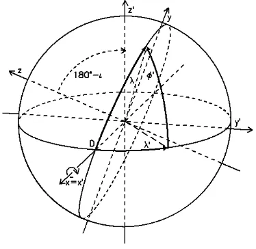
Figure 1. Rotation of coordinate system Σ around x axis with angle 180o - ι into Σ’
An orbit can be described by a Cartesian system Σ with one axis from the centre point through x=r, y=0, z=0 (r – semi major axis of orbit). This means in spherical coordinates that for crossing of x-axis by the orbit latitude and longitude are zero. The orbit is located in the oblique x-y plane (circle) of Figure 1 and its orientation to Sun is nearly constant during a day. When
the Cartesian system Σ rotates only around the x-axis with
180o - ι (ι - inclination of orbit) according Figure 1 the matrix elements for transformation (Mathematik, 1970) of equation (1) are reduced to the values shown in Table 2. In this case the orbit is crossing the x=x’ axis at the same “equator crossing” points in Σ and Σ’: (r;0;0) and (-r;0;0), respectively.
Table 2. Matrix elements of transformation equation of a Cartesian system Σ rotating with angle 180o - ι around the
x-axis into Σ‘
The Cartesian coordinates can be substituted by using spherical coordinates according equation (2):
x = r cosφ cosλ in spherical (geographical) coordinates angles φ’ (latitude) and λ’ (longitude) and the relation r = r’. Introducing these values including the coefficient aik of Table 2 into equation (1) the
following 3 relations can be derived:
cosφ' cosλ’ = cosφ cosλ
cosφ’ sinλ’ = - cosι cosφ sinλ + sinι sinφ (3)
sinφ’ = - sinι cosφ sinλ - cosι sinφ
where r’, φ’, λ’ = spherical (geographical) coordinates in Σ’
ι = angle between Σ and Σ’ after rotation around x-
axis (inclination of satellite orbit)
When using the ratio between second and third relation of equation (3) with the assumption that the latitude of the orbit in Σ is φ=0o the following relation can be found
cosφ’ sinλ’/ sinφ’ = cotι (4)
where φ’, λ’ = spherical (geographical) coordinates of
satellite orbit in Σ’
in which the longitude λ’ can be separated as given in equation (4).
λ’ = arcsin (tanφ’ cotι) (5)
Equation (5) can be solved for each longitude λ’ = λ’LC of local
crossing including the special case λ’ = λ’LEC = 0 of equator
Δλ’ = λ’LEC - λ’LC (6)
where λ’LEC = geographical longitude of local equator
crossing
λ’LC = geographical longitude of local crossing
The difference of the longitude in equation (6) is independent from Earth rotation, from geographic longitude of equator crossing and can be expressed as a time offset from the point of equator crossing to the orbit point of local crossing with equation (7).
toff = tLEC - tLC= Δλ’ / 15 = arcsin (tanφ’ cotι) / 15 (7)
where tLEC = LECT
tLC = LCT
After rearrangement equation (7) results in
tLC = tLEC - arcsin (tanφ’ cotι) / 15 (8)
Maximum and minimum of geographical latitude φ’ are determined by inclination of orbit. Its variation can be described by varying of λ in the third part of equation (3) with φ=0.
Equation (8) describes the relation for descending node (+ in case of ascending node) of the orbit as can be found already in Ignatov et al. (2004), Wu and McAvaney (2006). Equation (8) assumes that the daily actual value for LECT is used. In connection with equation (8) a relation of Local Time (LT) was used by Ignatov et al. (2004) and Wu and McAvaney (2006) at each geographic point for mean solar conditions given by e.g. Duffett-Smith (1988):
Because LCT is a synonym of LT in relation to orbit geometry, the combination of equation (8) and (9) gives the central geographic sampling positions of the LCT sampling method (Wu and McAvaney, 2006). Furthermore, if GMT and geographic longitude λ of the equator crossing are known or calculated (Ignatov et al., 2004), the result of equation (9) is a constant (mean) LECT, only influenced in case of NOAA satellites by drift of orbit connected with drift of LECT. Longitude of equator crossing and the corresponding crossing time in UTC (for our purpose UTC = GMT) are determined by Ignatov et al. (2004) for different satellites (NOAA, ERS, EOS) and for each day on basis of the two-line-elements (TLE), available for their full lifetime period and with help of Brouwer-Lyddane orbit prediction package (Kidwell, 1998, Goodrum et al., 2003). On basis of these results and use of equation (9) an equation for LECT will be determined describing the drift of LECT, with changing parameters from satellite to satellite. But as already mentioned, a difference exists between true and mean Sun. For example, local noon will change within -14 and +16 minutes within a year when using real Sun conditions. Neglecting the change of orbit parameters, LECT for real Sun will change for each satellite in the same order. This relation described by Equation of Time (ET) can also be found in Duffett-Smith (1988), and is caused by tilt of Earth axis and elliptical orbit of Earth around Sun. More details about this complex term are available e.g. in Duffet-Smith (1988) and
Smart (1949). For this purpose equation (10) for real Sun conditions has to be used instead of mean Sun conditions used in equation (9).
tL = tLC = tGM + tE + λG / 15 (10)
where tE = ET
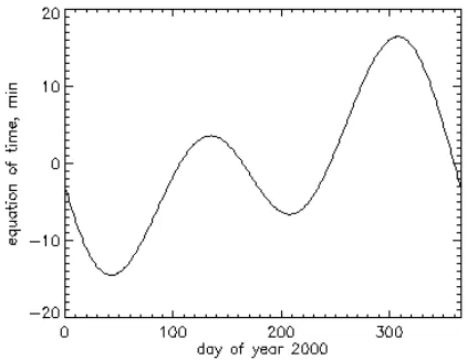
The ET variation computed for year 2000 is shown in Figure 3.
Figure 3. Variation of the difference between true and mean solar time calculated for year 2000
Because the calculation of ET is very complex, equation (11) represents an approximation for comparable purposes given in Baldocchi (2012) and Meeus (2000):
3600
Nominal ECTs (ECT at launch) including orbital drift rate of different NOAA satellites are given by Waliser and Zhou (1997) and Lucas et al. (2001). Mears et al., (2002) and Mears and Wentz (2009) have determined a global diurnal correction adjustment of temperature in their trend analysis, obtaining a similar annual behaviour as for the Equation of Time, but with different amplitudes. A variation of global adjustment of about 0.06 K within a year is shown in the corresponding results. It was shown that it is necessary to consider the long term drift of LECT, caused by slow changes in orbital parameters of each platform. Compared with these trends in changes of more than 3 hours during their life time e.g. NOAA-11 from 1989 to 1995 the influence of ET is small. Bush et al. (1999) show, that the long term trend of the local solar time of the ascending node of the NOAA-9 orbit is overlapped by the characteristic cycles of ET.
In many fields of geophysics the diurnal behaviour of time in Earth system is described with relation (10), for example when modelling the behaviour of minor constituents in neutral atmosphere (Fichtelmann and Sonnemann, 1989) for a geographic position depending on solar zenith angle. If LECT (tLEC) of a date is known (index 0), it is possible to
two different times (one with index 0), combining the corresponding two equations, and with view to orbit characteristic that tGM + λG /15 for sun-synchronous orbit of a
satellite, the difference between the two equations results after rearrangement in eq. (12).
tLEC = tLEC_0 + (tE – tE_0) (12)
where tLEC_0, tE_0 = LECT, ET for real Sun and defined day 0
tLEC, tE = LECT, ET for real Sun and a day of year
Possible disturbances as orbital drift have to be included into equation (12) additionally. The inclusion of tLEC of equation
(12) into equation (8) results in equation (13).
tLC = tLEC_0 + (tE – tE_0) - arcsin(tan(N) cotι) / 15 (13)
where tLC = LCT, ET for real Sun
N = geographic latitude in nadir view of satellite
ι = inclination of orbit
As shown before for some examples LECT for sun-synchronous satellites is given only for a mean value. This equation can be used to determine the actual ECT for real Sun conditions when using for tLEC_0 the corresponding mean value tLEC_MEAN together
with equation of time tE_0 of the same day.
Equation (13) only applies to the nadir point of the satellite orbit. Therefore, the local time for all pixels of an image line have to be corrected by using their respective length difference
= - N to the nadir point of this line by an additional term,
converting length difference into time difference according equation (14).
tLC = tLEC_0 + (tE – tE_0) - arcsin(tan(N) cot(ι)) / 15 + / 15
(14) where N = geographic latitude in nadir view of satellite
= difference of longitude from pixel in nadir view to a pixel in the same line
When using the ratio between first and second relation of equation (3) with the assumption that the longitude of the orbit in Σ is λ =0o the following equation (15) can be found.
λ’ = arctan (tanφ sinι) (15)
where = geographic latitude in Σ of Figure 1
λ’ =
For determination of mean LECT of LANDSAT 7 satellite the available TLEs and the STK orbit determination software (AGI, 2006) were used.
For demonstration of possible influence of ET to satellite products a LANDSAT 7 scene of 2nd June 2000 was used, as well as an atmospheric correction procedure according Holzer-Popp et al. (2004) in which the correct ET could be modified.
3. RESULTS
The result of calculation of toff in equation (7) for a complete
LANDSAT 7 orbit with an inclination ι=98.2degrees is given
with respect to the equator crossing of the descending node in Figure 4. The variation of toff is not only similar to results
described already by Johnson et al. (1994) for NOAA satellites. It is a characteristic feature of a sun-synchronous orbit. Knowing the actual (mean, real) ECT of descending node, the value can be added to the offset of this figure. Equation (8)
describes the dependency of (mean, real) LCT as function of actual latitude and the two orbit parameters tLEC and inclination
ι.
Figure 4. Time offset from LECT of descending node of LANDSAT 7 with an inclination of 98.2 degrees
The STK orbit determination software (AGI, 2006) was used to calculate mean LECT of LANDSAT 7 satellite in UTC on basis of the TLEs. The regular use of this software at acquisition facility in Neustrelitz has demonstrated over many years that a good agreement exists between calculated and real orbit parameters. Therefore we presupposed that the computation accuracy is well for calculating ECT. Ignatov et al. (2004) have pointed out, that their reconstruction of different past ECTs (TIROS-N, NOAA-6 through -17) was within an accuracy of ±2 min, using the same orbit determination software as mentioned before. The annual variation of equator crossing (mean LECT) of LANDSAT 7 platform was simulated for this paper by using NORAD orbit elements provided by CelesTrak ,within the System Tool Kit Software developed by Analytical Graphics, Inc. (AGI) for each 21st of all twelve months over year 2000. Equation (10) was used to transform ECT given in UTC (it corresponds to mean LECT) into LECT for real Sun.
Figure 5. Variation of LECT determined for each 21st day of a month, calculated by means of STK software of acquisition facility for mean (triangles) and real (asterisks, connected by dashed line) Sun of descending node of Landsat 7 for year 2000.
Variation of ET according equation (12) with ET of 21st June as
The calculated values of real LECT for descending node of LANDSAT 7 are shown by asterisks in Figure 5. Already with help of these 12 points it is obvious, that the variation of LECT for real Sun is very similar to that of ET in Figure 3. The nearest value to the 10:06 a.m. mean of these 12 values is given for the 21st of June. If using the tLEC_2106 and tE_2106 for this date as basis
(index 2106 instead of 0), it is possible to describe the annual variation of tLEC with equation (12). The result is given as solid
line in Figure 5. There is a good correspondence between these two curves but with increasing difference in the second part of the year. The third curve, the mean LECT (triangles) determined without consideration of ET shows a small decrease of LECT with a minimum in October and an increase in the last two months of the year. The maximum of deviation in year 2000 is around 2.5 minutes.
As can be seen in Figure 5, ET crosses four times (on days 107, 164, 245 and 360) the mean value of year 2000. It should be mentioned here, that a small change of crossing dates (also ET of a selected day) is possible, comparable with change of e.g. vernal equinox from year to year in Gregorian calendar (Duffet-Smith, 1988). In case, that LECT for real Sun (tLEC_0) is
available or can be determined for a day of year the variation of LECT for real Sun can be described by equation (13) without additional use of orbit determination software if the drift of orbit during life time of a satellite or time interval is with 2.5 min as found in our example with LANDSAT 7 in an acceptable order of magnitude for data users.
An automatic atmospheric correction (Holzer-Popp et al., 2004) was used to demonstrate in a single experiment the order of magnitude of influences of LECT variations caused by ET to Normalized Difference Vegetation Index (NDVI). For the purpose, two computations were carried out with the same LANDSAT-7 ETM+ dataset for the region of Mecklenburg-Western Pomerania (Germany) on 2nd June 2000. The first one was made under real LECT conditions including an ET of 1.93 minutes calculated for this date. The second one was carried out under simplified assumption. At first, to avoid changes of resulting parameters, e.g. NDVI, caused by changes of
vegetation within a year, the data set above was used as reference. Secondly a simulated time offset of 30 minutes based on real variability of ET between -14 min and + 16 min within a year was used. As mentioned before, if using one data set in minimum and another one in maximum of ET it is difficult to compare the results, e.g. on basis of NDVI, due to seasonal changes.
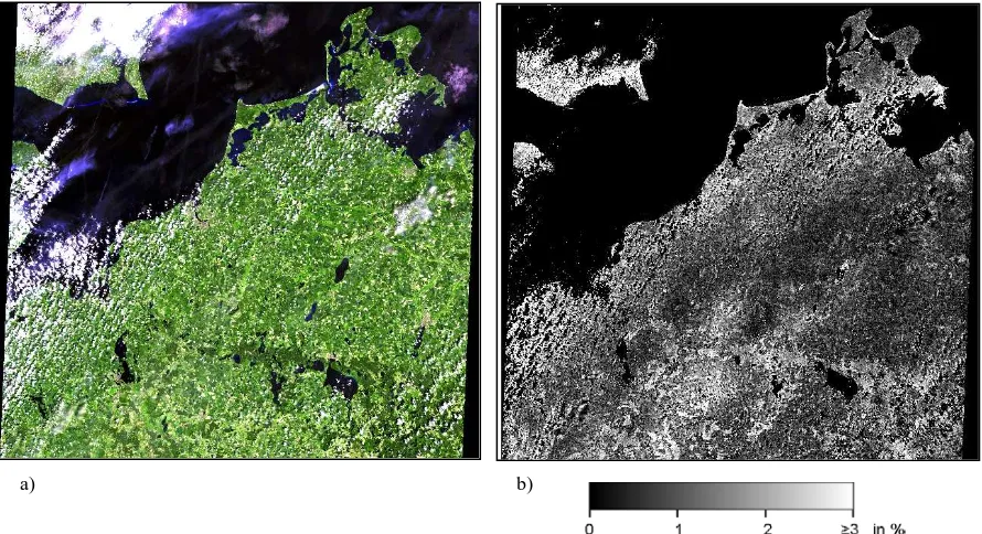
Figure 6 gives an estimation of the order of magnitude of the deviations of NDVI when using a mean LECT. Figure 6a shows the result in the RGB combination of ETM+ bands 7,5,3 after the automatic atmospheric correction using a pre-classification and real atmospheric data (ozone, water vapour and aerosol) of the same date. The relative difference of the NDVI (|NDVIoffset -NDVI|/NDVI) calculated with a hypothetical and without time offset, is shown in Figure 6b. Within the large and relatively dark region on the right side of Figure 6b the deviation (with some small exceptions) is consistently in the range of 0.5 to 1.5 %. In the lower centre, the deviation is in the order of 2.0 to 3.0 % and the cloud-free region in the upper left part (Denmark) shows deviations of up to 8 %.
4. DISCUSSION
The nearly constant ECT or corresponding LCT of a selected latitude is one of the important characteristics of sun-synchronous orbits. The term “nearly constant” includes small disturbances of the satellite orbit around the Earth and disturbances caused by the characteristics of Earth orbit around the Sun. The latter effect is connected with a seasonal variation of LECT of about ±15 minutes described by the Equation of Time. It was shown with the simple assumption of a 30 minutes time offset that the use of a mean LECT can have not only a strong influence to the results of automatic atmospheric correction but also on results based on these corrected optical data. It is assumed that atmospheric correction commonly includes the correct use of ET. Nevertheless, the inconsistence in determination of LCT was found with the use of the above Figure 6a and b. The region of Mecklenburg-Western Pomerania in an atmospheric corrected Landsat-7 dataset (rgb – ETM+
bands 7,5,3) on 2nd June 2000 with LECT for real Sun (a) in comparison with the relative deviation of NDVI when using a time offset for ET of 30 min .
formulas but without consideration of Equation of Time when no temporal information of a dataset was available.
It was already shown in studies about troposphere temperature that the long time drift of LECT can have an important influence on trend analyses of climate. Bush et al.(1999) are showing in their long term trend analysis of the local solar time of the ascending node of the NOAA-9 orbit the characteristic cycles of the equation of time. Mears et al. (2002) present in their studies about correction of MSU (Microwave Sounding Units) middle tropospheric temperature for diurnal drifts a global diurnal correction to 9 NOAA satellites between 1978 and 1999 with the characteristic behaviour of the ET. Therefore, concerning LST analysis, it is necessary to check whether the neglect of ET is resulting in a part of diurnal correction parameters. This part is in the order of magnitude up to 0.08 Kelvin as can be found in the results of Mears et al. (2002). The use of the equations for determination of LCT without consideration of ET was found in connection with simulation of radiances with the method of local-crossing-time sampling. For example, it is necessary to examine whether it is possible that the combination of the measured radiances with a small difference in LCT can result in small deviations of simulated brightness temperatures.
The results of a simplified change of correct use of ET show for example, that the influence on a value added product on basis of bottom of atmosphere reflectance as vegetation index NDVI is relatively small, but in some cases up to 8 %. The background is that the deviations for two used bands are going regularly into the same direction. On one side this paper shall convey an impression about the dimension of ET caused deviations in NDVI, which is connected with the atmospheric corrected values of one band. It should be noted here that already the calculation of top of atmosphere reflectance is required by more accurate calculation of Sun elevation. Studies of Jiang et al. (2008) show, that there is a dependency of NDVI magnitude on satellite ECT in the unadjusted global NDVI data set. Furthermore it was shown by Jiang et al. (2008) that one of the significant problems in the unadjusted NDVI time series on basis of NOAA satellites is the obvious dependency on satellite ECTs from different polar orbiters. But in some of the presented time series of unadjusted and adjusted NDVI the typical variation of ET within a year is obvious.
On the other side no reason was found why in the field of climatology the Equation of Time is not included. A lot of work has been done to determine the drift of LECT, e.g. Ignatov et al. (2004) have fitted the LECT drift by a mathematical approximation of a periodic function with one or two Fourier terms. It should be of advantage to use the complete formula of e.g. Duffet-Smith (1988) describing additionally the deviation between real and mean Sun.
A simple formula can be used to determine the actual LECT for real Sun within a year on basis of its value on a well defined date or on basis of a mean value given as orbit parameter and without inclusion of additional orbit determination software in the processing of data. In case of satellites with a drift during life time as NOAA satellites it is of advantage to eliminate ET from the mathematical description of such long time drift effects of equator crossing.
The determination of LECT of satellites with stabilized orbits as e.g. LANDSAT 7 shows for year 2000 a variation of about 2.5 minutes. Because the accuracy of time calculations is essential in Earth observation it would be of advantage when the actual LECT for real Sun will be included in the metadata of such a remote sensing product.
ACKNOWLEDGEMENTS
The authors wish to thank C. Wloczyk for her suggestions and advices.
REFERENCES
AGI, 2006, Analysis software for land, sea, air & space. 220 Valley Creek Blvd., Exton, PA 19341 USA, https://www.agi.com/ (23 Oct. 2012).
Aster Science Project, 2001. User’s guide, ERSDAC. http://www.science.aster.ersdac.jspacesystems.or.jp/en/documnt s/users_guide/part1/pdf/Part1_4E.pdf (23 Mar. 2015).
Baldocchi, Dennis. “Lecture 7, Solar Radiation, Part 3, Earth-Sun Geometry” September 10, 2012., http://nature.berkeley.edu/biometlab/espm129/notes/Lecture%2 07%20Solar%20Radiation%20Part%203%20Earth%20Sun%20 Geometry%20notes.pdf (20 Mar. 2015).
Borg, E., Fichtelmann, B., Asche, H., 2012. Design and implementation of data usability processor into an automated processing chain for optical remote sensing data. 5th International Symposium On Leveraging Applications of Formal Methods, Verification and Validation 15-18 October 2012 Amirandes, Heraklion, Crete, (oral presentation).
Bush, K.A., Smith, G.L., and Young, D.F., 1999. The NOAA-9 earth radiation budget experiment wide field-of-view data set. 10th Conference on Atmospheric Radiation, June 1999, NASA 1999 Technical Docs.
Duffet-Smith, P., 1988. Practical astronomy with your calculator. 3rd edn (Cambridge, N.Y., Port Melbourne, Madrid, Cape Town: Cambridge University Press).
ESA, 1992. ERS-1 Satellite Concept. Orbit Information https://earth.esa.int/web/guest/missions/esa-operational-eo-missions/ers/satellite (23 Mar. 2015).
Fichtelmann, B. and Sonnemann, G., 1989. On the variation of ozone in the upper mesosphere and lower thermosphere: A comparison between theory and observation, Z. Meteorol., 39, 297–308,
Goodrum, G, Kidwell, K., and Winston, W. (editors), 2003. NOAA–KLM User’s Guide. US Department of Commerce, NOAA/NESDIS. Available from National Climatic Data Center, 151 Patton Ave, Rm.120, Asheville, NC 28801-5001, USA.
Holzer-Popp, T., Bittner, M., Borg, E., Dech, S., Erbertseder, T., Fichtelmann, B., and Schroedter, M., 2004. Method for correcting atmospheric influences in multispectral optical teledetection data. European Patent Office, EP 1 091 188 B1,.
Ignatov, A., Lazlo, I., Harrod, E.D., Kidwell, K.B., and Goodrum, G.P., 2004. Equator crossing times for NOAA, ERS and EOS sun-synchronous satellites, International Journal of Remote Sensing, 25, 5255-5266.
ISRO, 2015. IRS-P6 / RESOURCESAT-1, http://www.isro.gov.in/Spacecraft/irs-p6-resourcesat-1 (23 Mar 2015).
in NOAA’s global vegetation index data sets, IEEE Transactions on Geoscience and Remote Sensing, 46, pp. 409-422.
Johnson, D.B., Flament, P., and Bernstein, R.L., 1994. High-resolution satellite imagery for mesoscale meteorological studies. Bulletin of the American Meteorological Society, 75, 5-34.
Julien, Y. & Sobrino, J. A. (2012). Correcting Long Term Data Record V3 estimated LST from orbital drift effects, Remote Sensing of Environment, 123 (2012) 207-219.
Julien, Y., Sobrino, J. A. & Jiménez-Muñoz, J.-C. (2011). Land use classification from multitemporal Landsat imagery using the Yearly Land Cover Dynamics (YLCD) method, International Journal of Applied Earth Observations and Geoinformation, 13 (2011), 711-720.
Kidwell, K. (editor), 1998. NOAA Polar Orbiter Data User’s Guide (TIROS–N, NOAA6, 7, 8, 9, 10, 11, 12, 13, and -14. US Department of Commerce, NOAA/NESDIS, 394 pp. Available from National Climatic Data Center, 151 Patton Ave, Rm.120.
LANDSAT Project Science Office, 1998. NASA’s Goddard Space Flight Center, Greenbelt, Maryland http://landsathandbook.gsfc.nasa.gov/data_prod/prog_sect11_3. html/ (20 Mar. 2015).
Lucas, L.E., Waliser, D.E., Xie, P., Janowiak, J.E., and Liebmann, B., 2001. Estimating the satellite equatorial crossing time biases in the daily, global outgoing longwave radiation dataset. Journal of Climate, 14, 2583-2605.
Mathematik, 1970. Kleine Enzyklopädie Mathematik. Ed.: Gellert, A., Küstner, H., Hellwich, M., Kaestner, H., 5th Ed. Verlag Enzyklopädie Leipzig.
Mears, A.M., Schabel, M.C., Wentz, F.J., Santer, B.D., and Govindasamy, B., 2002. Correcting the MSU middle tropospheric temperature for diurnal drifts. Proc. Int. Geophysics and Remote Sensing Symp., Volume III, Toronto, ON, Canada, IEEE, pp. 1839-1841.
Mears, A.M., Wentz, F.J., 2009. Construction of the remote sensing systems V3.2 atmospheric temperature records from the MSU and AMSU microwave sounders. Journal of Atmospheric and Oceanic Technology, 2009, Volume 26, pp. 1040-1056.
Meeus, Jean. 2000. Mathematical Astronomy Morsels, 2nd Ed. Willmann-Bell Inc.: Richmond, pp. 337-346
Mo, T., 2009. A study of the NOAA-15 AMSU-A brightness temperatures from 1998 through 2007. J. Geophys. Res. 114 D11110 doi:10.1029/2008JD011267 pp. 10.
Smart, W.M., 1949. Text-Book on Spherical Astronomy. Cambridge University Press, first edition 1931.
Sobrino, J.A., Julien, Y., 2013. Time series corrections and analyses in thermal remote sensing. In Thermal Infrared Remote
Sensing: Sensors, Methods, Applications, Remote Sensing and
Digital Image Processing, C. Kuenzer and S. Dech (Eds.), DOI 10.1007/978-94-007-6639-6_14, Springer Science+Business Media Dordrecht, 267-285.
Waliser, D.E., and Zhou, W., 1997, Removing satellite equator crossing time biases from the OLR and HRC datasets. Journal of Climate, 10, 2125-2146.