DEM RECONSTRUCTION USING LIGHT FIELD AND BIDIRECTIONAL
REFLECTANCE FUNCTION FROM MULTI-VIEW HIGH RESOLUTION SPATIAL
IMAGES
F. de Vieilleville a, *, T. Ristorcelli b, J.-M. Delvit c, a
MAGELLIUM SAS, Dept. Earth Observation, Ramonville-Saint-Agne, France, b
MAGELLIUM SAS, Dept. Imaging and Applications, Ramonville-Saint-Agne, France, {francois.devieilleville, thomas.ristorcelli}@magellium.fr
c
CNES, Dept. SIQI , Toulouse, France, [email protected]
Commission III, WG III/3
KEY WORDS: DSM reconstruction, BRDF, Light field, Image sequence
ABSTRACT:
This paper presents a method for dense DSM reconstruction from high resolution, mono sensor, passive imagery, spatial panchromatic image sequence. The interest of our approach is four-fold. Firstly, we extend the core of light field approaches using an explicit BRDF model from the Image Synthesis community which is more realistic than the Lambertian model. The chosen model is the Cook-Torrance BRDF which enables us to model rough surfaces with specular effects using specific material parameters. Secondly, we extend light field approaches for non-pinhole sensors and non-rectilinear motion by using a proper geometric transformation on the image sequence. Thirdly, we produce a 3D volume cost embodying all the tested possible heights and filter it using simple methods such as Volume Cost Filtering or variational optimal methods. We have tested our method on a Pleiades image sequence on various locations with dense urban buildings and report encouraging results with respect to classic multi-label methods such as MIC-MAC, or more recent pipelines such as S2P. Last but not least, our method also produces maps of material parameters on the estimated points, allowing us to simplify building classification or road extraction.
* Corresponding author
1. INTRODUCTION
Although an extensive body of literature over the subject of dense DSM reconstruction exists, the reconstruction of a reliable DEM or DSM from visible passive optics sensors is still a challenging task nowadays. In particular, occlusion problems, radiometric variations due to specular objects, shadows and precise localisation are at the core of these challenges. This is especially true on complex scenes such as dense urban areas since they gather all these difficulties. Looking at the height estimation of points on registered images, one usually cast the problem into a disparity estimation problem in a specific geometry. We thus seek the displacement for each pixel between two registered images. Depending on the chosen formulation, many methods exist to solve the problem. The solutions are often a trade-off between pure local radiometric matches (with estimation errors due to the image noise), global priors over the displacement map (varying smoothly, sharp edges, heavy-tail distribution, etc) and the step for the discrete estimation. Such problems are sometimes named “multi-label problems”, and graph-cut techniques (Boycov et al., 2001) seemed very promising although they only provided an estimation of the sought solution. Improvements were brought in specific cases (Ishikawa, 2003) which could be applied to disparity estimation. In this way, the work of (Pock et al., 2008; 2010) seemed even more promising for a global solution was provided, with less memory consumption, in a continuous framework solving a convex problem with higher dimension. Approximate solutions to non-convex problems are also sought with semi-global matching (Hirschmuller, 2008) which provides an efficient linear-time algorithm and very high visual quality results. Other algorithms try to bring an estimate through
filtering, such as volume cost filtering (Rhemann et al., 2011) using in this very special case additional information as a base for the support of the applied filters. On the other hand, when more than two images are used, most of these algorithms have to work on each or a few of couple images and then to decide which values are to be trusted. Other works have focused on using all the available information from the multiple views at the same time. The light field method (Kim et al., 2013) casts the disparity estimation problem on all views into a straight line seeking problem, which is very appealing when many views are available.
From a sensor point of view, a first problem comes from the fact that many satellites are not following a pinhole or projective geometry. Most of them are push-broom sensors and they do not follow the same geometric rules: epipolar lines become hyperbolas. However, recent studies from the CMLA (de Franchis et al., 2014a; 2014b; 2014c), on Pleaides imagery deal with adapting and correcting the push-broom geometry to use “on-the-shelf” computer vision disparity algorithms. To this end, they process the image on a tile-by-tile basis with location corrections to ensure that the approximation error of the hyperbolas remains within less than one tenth of a pixel.
So to some extent the push-broom sensor geometry is not an issue. What seems more troublesome is the variability of the radiometry when the same scene is viewed from different points of view. In fact, the only model usually implemented is the Lambertian one, which assumes that the luminance reflected by a surface only varies as a function of the angle between the normal to the observed point and the lightning direction, not the view direction. A simpler way to put it is that no radiometric
models are assumed when seeking disparities. Although this simple model is generally found in shape-from-shading algorithms, good results may follow (Courteille et al., 2004). In this paper we propose to address the radiometry problem using a non Lambertian bi-directional reflectance function (BRDF). We chose the classic Cook-Torrance parametric model and combined it with adapted light field approach inspired from the paper (Kim et al., 2013) so as to benefit from all the view. Moreover we want our output to be in the shape of a cost volume, to allow multi-label problem solving algorithms (graph-cuts, semi-global matching, volume cost filtering) to refine our results.
The remaining of the paper is organized as follow: in Section 2, we first recall the principles of the light field and the chosen illumination function, then we explain how to adapt light field methods with push-broom sensors and how to shape the output so as to use post-filtering methods. We also highlight the difference with respect to the existing light field method. In Section 3, we present our dataset, first results, and some state-of-the-art DSM on the same scene. A discussion on the results obtained and the method follows in Section 4. Eventually we conclude on the possible improvements of the method and some of its possible uses.
2. LIGHT FIELD, ILLUMINATION AND PROPOSED METHOD
We first describe the light-field approach and its requirements. Then, we move to the selected illumination model its implementation within the light-field method. Eventually, we elaborate on the required shape of the output in a suitable way for state-of-the art post processing.
2.1 Light field
(Bolles et al., 1987) describes the following requirements for light field imagery:
1) the camera movement is rectilinear at constant speed, 2) each acquisition is separated by the same amount of time (regular sampling),
3) the camera point of view is perpendicular to the movement direction.
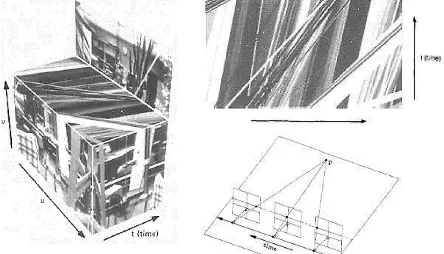
Figure 1. Illustration of the light field requirements, epiplanar slice of the epibloc and epibloc (Bolles et al., 1987).
Considering a couple of consecutive images for a given feature, the relation between the distance and the camera path (D) depends on the focal distance of the camera (h), the distance between the acquisition (ΔX) and the observed displacement of the feature on the images (ΔU):
When these requirements are met, a given feature on an image is moving along the horizontal direction U. The apparent velocity of the feature displacement only depends on its distance with respect to the moving direction of the camera. From an image point of view, stacking the acquired images provides a 3D volume, slicing it along the U and time direction brings a plane on which features displacements are lines with different slopes, see Figure 1 for an illustration.
U X h D
* (1)
Using these principles (Kim et al., 2013) have designed a bottom-up approach identifying the most probable recognized lines based on simple filtering of the radiometry and edge estimation for the selection of the points on which to perform the line recognition at each scale. In fact, one drawback of the epiplanar representation is that features at similar height belonging to a same neighborhood and having similar radiometry may appear as a band of a given thickness, entailing an uncertainty on the recognized slope of the line. This is particularly visible on spatially homogeneous image patches, as illustrated on Figure 2.
Figure 2. An image zone (U,V) with a homogeneous roof and the epiplanar slice (U, Time) associated to the yellow line. The possible uncertainty of the slopes clearly depends on homogeneity of the roof. Since the sensor motion is neither rectilinear nor at constant velocity, lines are in a wedge shape form.
The classic light-field algorithm assumes that an object appears in the image sequence with the same radiometry. This hypothesis is reasonable if the incidence variations are within a few degrees of range. However, in the case of a satellite sequence, viewing angles range from -45° to 45°. In that situation, the Lambertian hypothesis is not suitable anymore.
2.2 Illumination model
A popular and generic way of describing light reflection on a hard surface is the bi-directional reflectance function (BRDF). The BRDF is defined as the ratio between exiting radiance and incoming irradiance, and accounts for all angular dependencies.
)
(
)
(
)
,
(
i i
r r r i r
dE dL f
(2)Under the Lambertian hypothesis, the BRDF is the constant:
, )( i r
BRDF (3)
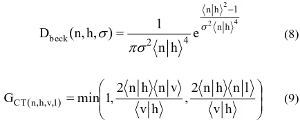
where ρ is the surface reflectance (or albedo), i.e. the ratio between total reflected and incoming energy. Many BRDF models have been developed that are capable of accounting for non-Lambertian behaviors. For our light field approach, we selected the Cook-Torrance model (Cook and Torrance, 1981), with the Schlick approximation in the Fresnel term (Schlick, 1994).
Figure 3. Illustration of the Cook-Torrance surface reflectance for increasing roughness.
This reflectance function is the sum of two contributions, a pure Lambertian term and a micro facet term producing a semi-specular reflection. The second term is obtained by modelling the surface as pure specular elementary facets, whose geometric orientation follows a given distribution, see
Figure 3 for an illustration. The exact used formulations can be found thereafter:
With l being the normed lightning vector, v the normed viewing vector, kl, η and σ being respectively the Lambertian coefficient,
the refraction index and the roughness. All these values are to be considered for the observed point P and its geometry (in particular, its unitary normal vector). The micro-facets term is itself a product representing several parameters:
normed half-vector between l and n. Schlick’s approximation for the Fresnel term is the following and uses n as the refraction index.
The Beckmann distribution of the facets and the geometry term use n as the unitary normal vector at point P:
parameters involved. Using the satellite meta-data that come with the images, several parameters are known for each images, in particular the viewing direction and the lightning direction. To sum-up, the parameters to estimate for each imaged ground point is:
-The surface orientation (normal vector n) -The Lambertian reflectance kl
-Cook-Torrance parameters and n (surface roughness and refraction index)
We hereafter denote by ϴ this set of parameters, possibly indexed for U, V coordinates.
2.3 Proposed method
We will now describe our method explaining the extensions that were brought to the light field approach.
2.3.1 Geometric and time frame corrections: It is clear that in the general case of push-broom imaging the two geometric requirements from section 2.1 are not met. However, using a re-projection of the images, after refining through Euclidium, see (Magellium, 2013b), on a plane with constant height, we get images having the very same epipolar lines. Stacking them in sampling order, and slicing them in the (U, time) plane, we get an epipolar plane such as the one shown on Figure 4
5
Figure 4. Slice in the Epi-bloc along the (U,Time) direction for a given point along the V direction.
Now, we have to compensate for the time acquisition of the image since they were sampled on a non-rectilinear path, the path of a feature point (e.g. the corner of a building) is not a line. On our data, a Pleiades acquisition on Melbourne, we get a specific curve for each feature point, as illustrated on Figure 4. To correct this effect, we have to apply a time shift for each frame. This correction is computed with simple geometry relations with respect to the satellite path and the time between each acquisition. For practical purposes, we assume that our time frame indices span from 1 to 17. Eventually we get a simple formula for the location of a point on each frame from the U, V coordinates of a point on the nadir frame, its associated slope and multiplicative correction coefficients, denoted c:
With this, we get all the observed radiance on each frame for a given point at a supposed slope. This observation is shaped in a 1D 17 real valued vector, using a possible frame-wise resampling in the U dimension. We hereafter denote obs(u, v, s) such a vector. Assuming we have a merit function for a such a vector, spanning a given slope interval for a given point allows
us to determine, from the merit function point of view, its associated slope, thus enabling us to get its height.
2.3.2 Inverting the illumination function: The inversion is casted in a simple least square problem, that is:
2 randomly draw a starting point belonging to an admissible set of parameters. For each starting point a gradient descent scheme using various fixed step size, spanning from 10-9 to 10-1, is applied. Usually 100 iterations are enough to reach an acceptable approximation. Thanks to this method, we produce a cost volume corresponding, for each point seen in the central (nadir) frame and for a set of slopes, to the residual obtained when trying to fit the BRDF model to the 17 samples data.
Note that, in general, for sequence with high base over height ratio, multiple occlusion problems arise since only the highest points should be visible on all views. Iterative solutions exist (Kim et al., 2013) but with much more samples and a smaller base over height ratio. Due to time-consuming computations, we could not afford an iterative strategy were the visibility mask of each imaged point could be estimated. Consequently, we kept it to a minimum of three sets of profiles:
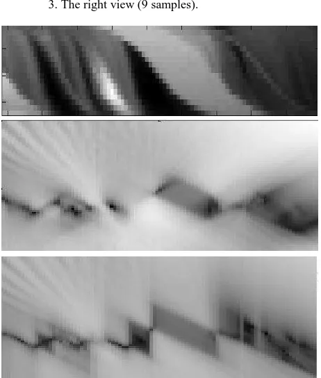
1. The full view for the highest points (17 samples) 2. The left view (9 samples)
3. The right view (9 samples).
Figure 5. Top: epiplanar slice in the (u,t) direction. Middle: profiles for each element at position (u, v, s). An illustration of
two profiles associated to a given epiplanar slice is provided on Figure 5.
2.3.3 Filtering/selection on the cost volume: As mentioned earlier, we output a merit function for each tested slope on each point of the nadir image. We thus collect a volume whose total number of element equals to the number of pixels along the U direction times the number of pixels along the V direction times the number of slopes that were tested. It is usually better to try slopes separated by a fixed amount. This amount shall be such that it is greater than one pixel on the extreme views.
Once the whole cost volume is computed we aim at assigning a slope index for each point (u, v) thus constructing an optimal surface. A naive strategy is to take the minimum along the slope direction for each point of the nadir image. This solution brings very noisy slope maps since a very precise visibility of each point has not been estimated and the associated residues lead to errors in the slope estimation. This problem is often encountered in computer vision literature. We have tested several state-of-the-art algorithms to be used with our cost volume, namely:
1. Semi-global matching (SGM), 2. Volume cost filtering, 3. Variational approach.
Let us describe very briefly these three methods:
Semi-global Matching (SGM)
This method is used for disparity estimation in stereoscopic imagery. Starting with disparity costs (radiometric) for each displacement for each epipolar lines it propagates the sum of the cost of a best path for each disparity. This is done by choosing the minimum over several candidates for the evaluation of the current disparity while propagating along an epipolar direction:
1) an adjacent neighbor plus a fixed cost (P1)
2) the previous cost along the line (same disparity) 3) the minimum cost for the previous points plus a second constant cost (P2).
This method then iterates in non epipolar directions, enabling a spatial regularization of the disparities using a non-convex regularization. In our case this method relies on a simple propagation of costs along a given direction in the (U, V) plane. Here, along the (1, 0) direction we get: (Hirshmuller, 2008). In our case, we only applied the first eight directions. Once the new volume cost is computed, we take the minimum along the slope direction for each (u,v) point.
Volume Cost Filtering
This method relies on local filtering of the costs in the spatial dimensions. For each point, a weighted sum over the spatial
neighboorhood is performed. The weights depend on an image relevant image, which, in our context, could not be found.
Variational Approach
In this method, we aim at finding the slope S for each point (u,v). As input, we use our cost volume here denoted ρ and a global prior over the field. The Total Variation prior was selected to allow sharp discontinuities in the final slope field, the resulting problem is:
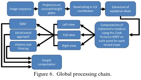
variable in a different space turning it in a “min max” convex optimization problem as explained in (Pock et al., 2008) and (Pock et al., 2010). We here directly get the best slope estimation once a stop condition is met (usually a given number of iteration).2.3.4 Global pipeline: We here sum-up the various processing that were used in this chain.
Figure 6. Global processing chain.
3. DATA SET, RESULTS, COMPARISON AND DISCUSSION 2012) for a better overview of the Pleiades satellite.
Figure 7. Illustration of the Melbourne Pléiades sequence, on first, nadir and last image. All these were reprojectedon a plane with constant height, the attitude were corrected through refining using Euclidium.
A preprocessing was first used on the images to set them in reflectance instead of a radiance digital count. Calibration coefficient, solar radiance and sun direction required to operate this computation were found in the meta-data. A global trivial surface normal was used in the process, as shown on Equation 16, where Xradio count stands for the radio count, G for the
calibration coefficient of the panchromatic band and Lin for the
sun irradiance: Figure 8, which consists of a set of high buildings and trees. We recall that the whole image sequence was used in the height estimation. However we have focused on a patch of size 1000x200 due to very high computation times.
More than 200 slopes were tested, with the upper and lower volume cost filtering on this specific scene, and all our attempts resulted in over smoothing of the height. The results appear to be noisy or inaccurate on homogeneous areas and in shadow areas, the regularizations helps to prevent large discrepancies.
Figure 8. Nadir view for our test scene, the image dynamic was slightly changed to make details more visible.
Figure 9. our method with the variational optimization.
Figure 10. our method with the SGM filtering
3.3 Comparison
The comparison here cannot be done on ground truth since, no lidar acquisition were available on the studied area. We thus just visually compare with some existing solutions. First with S2P2 CNES solution on the same region using a Pléiades triplet:
Figure 11. Results with the S2P2 pipeline.
Then with another solution from our company, see (Magellium, 2013a) for more details, still with a Pleiades triplet:
Figure 12. Results with the OrthoAdjust pipeline.
Obviously the S2P2 pipeline gives better results, however we note that the edges on the buildings seems quite sharp on our method, especially when the SGM filtering is used.
4. DISCUSSION
From the previous results and experiments, it is clear that the main drawback of our method is its computation time. In fact the optimization process to estimate the BRDF parameter from the observed samples should be done in a more efficient way. For example, a first guess could be done for the parameter based on the observed samples (from learning or classification methods) and then a descent gradient algorithm should refine the estimated parameters. Another huge optimization would be to have a guess for the slope values or at least to narrow the range of sought slopes. Such a range could be derived from a
low-resolution reference MNT, such as the NASA SRTM database. Another choice would be to maximize the alignment of the structure tensor in the epiplanar slices. Another important drawback of our algorithm is its weakness over the homogeneous areas since the variation of their reflectance on the image sequence is very small which entails ambiguous slope choices. Although the regularization helps in this matter, as all the possible choices have more or less the same residue value in the cost volume, it is still only a global prior. In the shadow zones, our BRDF model itself is not relevant since simplifications (e.g. punctual light source at infinity) were made, maybe simpler models on these areas would perform better.
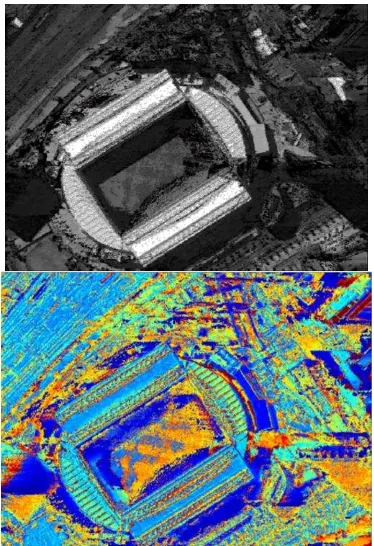
On the other hand, the parameters obtained from the inversion could be reused in segmentation/classification algorithms, although we have not investigated this matter, the obtained maps seems promising, especially on specular areas due to metallic part, see Figure 13 for an example.
Figure 13. (Top) Lambertian map obtained from the BRDF inversion. (Bottom) Roughness maps obtained from the BRDF inversion. Most of the blue zone underline observed specular behaviour.
5. CONCLUSION
To conclude, in this study we have provided a way to enlarge light field methods on non-pinhole sensors with non-rectilinear motion using a BRDF model. Although our test case only consists of 17 images, which are very hard conditions for a light field approach, the nominal case for DSM production is in general restricted to 3 or even 2 images of the same scene. More is to be done to speed up the computations or at least to reduce the required number of tested slopes. On the other hand the BRDF parameter extraction could lead to relevant classification/segmentation of the observed materials. Future work will focus on the reduction of the number of the required views and on a more in depth comparison and evaluation of the produced results.
REFERENCES
Bolles, R.C., Baker, H., and Marimont, D.H., "Epipolar-Plane Image Analysis: An Approach to Determining Structure from Motion", International Journal of Computer Vision, Vol. 1, No. 1, 1987, Kluwer Academic Publishers, pp.7–55.
Boykov, Y., Veksler, O., Zabih, R., “Fast Approximate Energy Minimization via Graph Cuts”, IEEE transactions on Pattern Analysis and Machine Intelligence (PAMI), Vol. 23, No. 11, pp.1222-1239, 2001.
Cook, R. L., and Torrance, K. E., “A Reflectance Model for Computer Graphics”, Computer Graphics, Vol. 15, No. 3, August 1981
Courteille, F., Crouzil, A., Durou, J. –D. and Gurdjos, P, "Towards Shape from Shading under Realistic Photographic Conditions," In Pattern Recognition, International Conference on, pp. 277-280, 17th International Conference on Pattern Recognition (ICPR'04) - Volume 2, 2004
de Franchis, C., Meinhardt-Llopis, E., Michel, J., Morel, J. M. and Facciolo, G., "Automatic sensor orientation refinement of Pléiades stereo images," Geoscience and Remote Sensing Symposium (IGARSS), 2014 IEEE International, p.1639-1642, 2014.
de Franchis, C., Meinhardt-Llopis, E., Michel, J., Morel, J. M. and Facciolo, G, "On stereo-rectification of pushbroom images," Image Processing (ICIP), 2014 IEEE International Conference on, pp.5447-5451, Paris, 2014.
de Franchis, C., Meinhardt-Llopis, E., Michel, J., Morel, J. M. and Facciolo, G., “An automatic and modular stereo pipeline for pushbroom images”, ISPRS Annals of Photogrammetry, Remote Sensing and Spatial Information Sciences, Vol. 2, No. 3 pp.49-56, 2014.
Hirschmuller, H., "Stereo Processing by Semiglobal Matching and Mutual Information," in IEEE Transactions on Pattern Analysis and Machine Intelligence, Vol. 30, No. 2, pp.328-341, Feb. 2008.
Ishikawa, H., "Exact optimization for Markov random fields with convex priors," in IEEE Transactions on Pattern Analysis and Machine Intelligence, Vol. 25, No. 10, pp. 1333-1336, Oct. 2003.
Kim, C. Zimmer, H., Pritch, Y., Sorkine-Hornung, A., Gross , and M.,”Scene Reconstruction from High Spatio-Angular Resolution Light Fields”, July 22, 2013, ACM SIGGRAPH 2013.
Kubik, P., Lebègue, L, Fourest, S., Delvit, J.-M., de Lussy, F , Greslou, D. and Blanchet G., “First inflight results of Pleiades 1A innovative methods for optical calibration”, International Conference on Space Optics, 2012Nicodemus, F., "Directional reflectance and emissivity of an opaque surface", Applied Optics Vol. 4, No.7 pp.767–775, 1965.
Magellium, 2013, “OrthoAdjust”, Toulouse, France, http://www.magellium.com/fr/blog/portfolio-item/orthoadjust-2/ (04 Mar. 2016)
Magellium, 2013, "Euclidium", Toulouse, France, http://www.magellium.com/fr/blog/portfolio-item/euclidium-2/ (04 Mar. 2016)
Pock, T., Schoenemann, T., Graber, G., Bischof, H. and Cremers, D., “A Convex Formulation of Continuous Multi-label Problems”. in 'ECCV (3)' , pp.792-805, 2008.
Pock, T., Cremers, D., Bischof, H. and Chambolle, A. “Global Solutions of Variational Models with Convex Regularization”, SIAM Journal on Imaging Sciences, Vol. 3, No. 4, pp.1122-1145, 2010.
Rhemann, C., Hosni, A., Bleyer, M., Rother, C., and Gelautz, M, “Fast Cost-Volume Filtering for Visual Correspondence and Beyond” Computer Vision and Pattern Recognition (CVPR), 2011 IEEE Conference on, 2011, pp. 3017-3024.
Schlick, C., “An Inexpensive BRDF Model for Physically-Based Rendering“, Proc. Eurographics’94, Computer Graphics Forum, Vol. 13 Number 3, pp.233-246, 1994