FLEXSIM SIMULATION TUTORIAL
Aliq Zuhdi
Kuliah Pemodelan Sistem - Program Magister Teknik Industri -
Universitas Islam Indonesia
Flexsim Concepts
Before you start this model it will be helpful to understand some of the basic terminology of the software.
Flexsim objects
Flexsim objects simulate different types of resources in the simulation. An example is the Queue object, which acts as a storage or buffer area. The Queue can represent a line of people, a queue of idle processes on a CPU, a storage area on the floor of a factory, a queue of waiting calls at a customer service center, etc. Another example of a Flexsim object is the Processor object, which simulates a delay or processing time. This object can represent a machine in a factory, a bank teller servicing a customer, a mail employee sorting packages, an epoxy curing time, etc.
Flexsim objects are found in the Library Icon Grid.
Flowitems
Flowitems are the objects that move through your model. Flowitems can represent parts, pallets, assemblies, paper, containers, telephone calls, orders, or anything that moves through the process you are simulating. Flowitems can have processes performed on them and can be carried through the model by material handling resources. In Flexsim, flowitems are generated by a Source object. Once flowitems have passed through the model, they are sent to a Sink object.
Itemtype
The itemtype is a label that is placed on the flowitem that could represent a barcode number, product type, or part number. Flexsim is set up to use the itemtype as a reference in routing flowitems.
Ports
Every Flexsim object has an unlimited number of ports through which they communicate with other objects. There are three types of ports: input, output, and central.
Input and output ports are used in the routing of flowitems. For example, a mail sorter places packages on one of several conveyors depending on the destination of the package. To simulate this in Flexsim, you would connect the output ports of a Processor object to the input ports of several Conveyor objects, meaning once the Processor (or mail sorter) has finished processing the flowitem (or package), it sends it to a specific conveyor through one of its output ports.
Central ports are used to create references from one object to another. A common use for central ports is for referencing mobile objects such as operators, fork lifts, and cranes from fixed resources such as machines, queues, or conveyors.
1) By clicking on one object and dragging to a second object while holding down different letters on the keyboard. If the letter 'A' is held down while clicking-and-dragging, an output port will be created on the first object and an input port will be created on the second object. These two new ports will then be automatically connected. Holding down the 'S' key will create a central port on both objects and connect the two new ports. Connections are broken and ports deleted by holding down the 'Q' for input and output ports and the 'W' key for central ports. The following table shows the keyboard letters used to make and break the two types of port connections. Lesson 1 of the tutorial demonstrates how to properly make port connections.
2) By entering the connection mode by clicking the button. Once in the connection mode, there are a couple of ways to make a connection between two objects. You can either click on one object, then click on another object; or you can click and drag from one object to the next as with method one. Either way, keep in mind that the flow direction of a connection is dependent on the order in which you make the connection. Flow goes from the first object to the second object. Incidentally, connections can be
broken by clicking the button then clicking or dragging from one object to another in the same manner as when you connected them. Center port connections need to be
Output - Input Center
Disconnect Q W
Connect A S
Lesson 1
Introduction
Lesson 1 introduces the basic concepts of diagramming and building a simple model. Building a diagram of the process is a great way to start every model that you will build in Flexsim. If you can not build a diagram, flowchart, or at least see a picture in your mind of how the process works, you will have a difficult time building the model in Flexsim.
Note: if you have already gone through the Getting Started tutorial, many of the concepts you learn in this lesson will not be new. However, subsequent lessons build upon this lesson, so it is probably a good idea to go through it anyway.
What You Will Learn
How to build a simple layout
How to connect ports for routing flowitems
How to detail and enter data into Flexsim objects
How to navigate in the animation views
How to view simple statistics on each Flexsim object
New Objects
Approximate Time to Complete this Lesson
This lesson should take about 30-45 minutes to complete.
Model views:
Flexsim uses a three-dimensional modeling environment. The default model view for building models is called an orthographic view. You can also view the model in a more realistic perspective view. It is generally easier to build the model's layout in the orthographic view, whereas the perspective view is more for presentation purposes. However, you may use any view option to build or run the model. You may open as many view windows as you want in Flexsim. Just remember that as more view windows are opened the demand on computer resources increases.
Model 1 Description
In our first model we will look at the process of testing three products coming off a
manufacturing line. There are three different flowitem itemtypes that will arrive based on a normal distribution. Itemtypes will be uniformly distributed between itemtypes 1, 2, and 3. As flowitems arrive they will be placed in a queue and wait to be tested. Three testers will be available for testing. One tester will be used for itemtype 1, another for itemtype 2, and the third for itemtype 3. Once the flowitem is tested it will be placed on a conveyor. At the end of the conveyor the flowitem will be sent to a sink where it will exit the model. Figure 1-1 shows a diagram of the process.
Model 1 Data
Source arrival rate: normal(20,2) seconds Queue maximum size: 25 flowitems Testing time: exponential(0,30) seconds Conveyor speed: 1 meter per second
Step-By-Step Model Construction
Building Your First Model
Open the application by double clicking on the Flexsim icon on your desktop. Once the software loads, you should see the Flexsim menu and toolbars, Library, and Orthographic Model View windows.
If at any time you encounter difficulties while building this model, a fully functional tutorial model can be found at http://www.flexsim.com/tutorials
Step 1: Create the Objects
Create a Source in the model and name it Source (To see how this is done, click here).
Create a Queue, 3 Processors, 3 Conveyors, and 1 Sink in the model. Place and name them as shown below. To name an object: double click on it, change its name at the top of the Properites window, and press Apply or OK. Click Here to see how this is done
Step 2: Connect the ports
Enter the connection mode by either clicking the button, or by pressing and holding the A key on the keyboard. Once in the connection mode, there are a couple of ways to make a connection between two objects. You can either click on one object, then click on another object; or you can click and drag from one object to the next. Either way, keep in mind that the flow direction of a connection is dependent on the order in which you make the
Incidentally, connections can be broken by clicking the button, or by pressing and holding the Q key on the keyboard, then doing the same as if you were connecting them.
Connect Source to Queue.
Connect Queue to Processor1, Processor2, and Processor3.
Connect Proceesor1 to Conveyor1, Processor2 to Conveyor2, and Processor3 to Conveyor3.
Connect Conveyor1, Conveyor2, and Conveyor3 to Sink.
Step 3: Assign the arrival rate
In this model we need to change the Inter-Arrival time and the itemtype to generate 3 types of items.
Double click on the Source to open its Properties window
On the Source tab, select Statistical Distribution from the Inter-Arrivaltime list. The code template window and a suggestion window will appear.
Double click normal(0, 1, 0). Then change the blue text as follows: Statistical Distribution: normal(20, 2, 0)
The next thing we need to do is assign an itemtype number to the flowitems as they enter the system. This will be uniformly distributed between 1 and 3. The best way to do this would be to change the itemtype on the OnCreation trigger of the Source, so don't close the Properties window yet.
Step 4: Set Itemtype and Color
Click the Triggers tab, and add a function (click the button) to the OnCreation trigger and select the Set Itemtype and Color option. The code template window will appear.
The duniform distribution is similar to a uniform distribution except that instead of returning any real number between the given parameters, only discrete integer values will be returned. The default blue text will be used in this example.
The next step will be to detail the queue. Since the queue is a place to hold flowitems until they can be processed at the processor, there are 2 things we need to do. First, we need to set the capacity of the queue to hold 25 flowitems. Second, set the flow options to send itemtype 1 to processor 1, itemtype 2 to processor 2, and itemtype 3 to processor 3.
Step 5: Setting the Queue Capacity
Double-click on the queue to open it's Properties window.
Change the Maximum Content to 25.
Step 6: Define the Flow for the Queue
Click the Flow tab in the Properties Window to set the flow options for the queue.
Since we have assigned an itemtype number equal to 1, 2, or 3, we can now use the itemtype to specify the port number through which flowitems will pass. Notice that the default output port is: getitemtype(item). Leave this as it is. Processor 1 should be connected to port 1, processor 2 should be connected to port 2 and so on. Click outside of the box to apply the trigger.
Click the OK button to close the queue's properties window.
The next step is to set the processor times
Step 8: Define the Process Time
Double-click Processor1 to open it's Properties window.
On the Processor tab, in the Process section, select Statistical Distribution from the Time list. The template window and the suggestion box will appear.
Double click exponential(0, 1, 0) in the suggestion box. Edit the blue text to read as follows
Statistical Distribution: exponential(0, 30, 0)
The default speed for the conveyors is already set to 1 length unit per time unit so there is no need to modify the conveyors at this time.
Now we are ready to run the model.
Step 8: Reset and Run the model
Always click the button to reset system and model parameters to their initial state before running a model.
Click the button to start the simulation.
Step 9: Viewing simple statistics
The above image shows how to view simple statistics for each object. If nothing is showing or only the names are showing, you can change the View Settings to show the statistics. To change the View Settings, right-click the background of the view and go to View > View Settings > Show Names and Stats.
Step 10: Save Model
Save your model by clicking the Save button on the main toolbar. The "Save Flexsim Model file" window will appear allowing you to navigate to the folder where you want to save your model. Change the "File name" to an appropriate name (lesson1.fsm) and select save.
Remember that the file name extension must be .fsm.
Lesson 2
Introduction
Lesson 2 introduces the concept of adding operators and transporters to a model, and explores object properties in greater detail. Lesson 2 also introduces additional graphical statistical output options. Make sure you have completed lesson 1 before starting lesson 2 as lesson 2 will use the model from lesson 1 as a starting point.
What You Will Learn
How to access and modify object properties
How to add a team of operators to the model
How to add a fork truck transporter to the model
How to select an object for graph data statistics
How to turn on stats collecting
How to view object statistics while the model is running
New Objects
In this lesson you will be introduced to the Dispatcher, Operator, and Transporter objects.
Approximate Time to Complete this Lesson
This lesson should take about 30-45 minutes to complete.
Model 2 Overview
In model 2 we will use a team of operators to perform the setup for the testing procedure for the flowitems in the model. One of two operators will need to set up the test. Once set up, the test can run without the need for the operator to be present. The operators must also carry the flowitem to the test station before the setup can begin. When the test is complete, the
flowitem moves to the conveyor without the assistance of the operator.
Model 2 Data
Tester set-up time: Constant time of 10 seconds
Product handling: Operator from queue to tester. Fork truck from conveyor queue to sink.
Conveyor Queue: Capacity=10
New Concepts
Object Properties
It is now time to introduce the object Properties window in a more organized manner. Every Flexsim object has a properties window. To access properties you can either double-click on an object or right-click on an object and click Properties
Step 1: Selecting objects for stats
In the model view window you will need to make a selection of objects for which you would like to record stats. This is done by holding the "Shift" key on the keyboard while dragging the mouse to include the objects you want to select. This can also be done using the New Selection mode on the Mode Toolbar. Pressing the "Ctrl" key and then clicking an object adds or removes individual objects from the selection set.
Step 2: Stats On
To gather stats histories on the selected objects, click on Statistics > Object Graph Data > Selected Objects On.
You can now run the model and collect stats histories on all objects that were selected.
This ends the Flexsim software concept learning section. It is now time to build model 2.
Step-By-Step Model Construction
Building Model 2
To start building model 2 you will need to load model 1 from the previous lesson.
If at any time you encounter difficulties while building this model, a fully functional tutorial model can be found at http://www.flexsim.com/tutorials
Step 1: Load model 1
If you do not have Model 1 open, load it by clicking the button on the toolbar. Select the file for model 1 (.fsm file) saved from lesson 1.
Step 2: Create a dispatcher and 2 operators
The Dispatcher is used to queue up task sequences for a team of operators or transporters. In this case it will be used with 2 Operators that will be used to move flowitems from the queue to the testers.
Create a Dispatcher and name it Dispatcher.
Step 3: Connect the Dispatcher and Operators
The queue is going to request an operator to pick up the flowitem and take it to one of the testers. The flow logic has already been set on the queue in lesson 1. You will not need to change the flow logic. You will only need to request an operator to be used for the task. Since we are using 2 operators, we will use a dispatcher to queue the requests and send them to a free operator to perform the task. If we only had 1 operator, we would not need the dispatcher and could connect the operator to the queue directly.
In order to use the dispatcher to direct a team of operators to perform a task, the dispatcher must be connected to the central port of the object requesting the operator. The central port is located in the center bottom position of the object. To connect the central port of the
dispatcher to the queue, press and hold the "S" key on the keyboard and then click-and-drag from the dispatcher to the queue. When you release the mouse button a connection from the dispatcher's central port will connect to the central port of the queue. You can also use the Connect Center Ports mode from the Mode Toolbar to do this.
In order for the dispatcher to send tasks to the operators, the dispatcher's output ports needs to be connected to the operators' input ports. This must be done for each operator.
Connect Queue to Dispatcher with a center connection (S key).
Step 4: Modify Queue Flow to Use Transport (Operators)
The next step is to modify the Queue's flow parameters so it uses the operators.
Double-click Queue to open its Properties window.
Click the Flow tab
Check the Use Transport box. The Request Transport From list will become available. This pick list allows you to select which Transporter or Operator to move the item based on the center port number. In this case it is the object connected to center port 1 (the Dispatcher) that assigns the operator to the task, so the default settings will work here.
Step 5: Save the Model, and Test Run
Now we should run the model to make sure that the changes we have made are working.
Reset the model and then Save the model by clicking the button on the toolbar.
Run the model to verify that the operators are moving the flowitems from the queue to the testers.
Step 6: Using Operators for the Process Setup Time
In order for the testers to use the operators during set up, a connection must be made between the central ports of each tester to central ports of the dispatcher. Then the setup time needs to be defined for the Processors.
Connect Dispatcher to Processor1, Processor2, and Processor3 with center connections (S key).
Double-click Processor1 to open it's Properties window.
On the Processor tab, under Setup, check Use Operator(s) for Setup. Number of Setup Operators and Pick Operator will become available.
Select By Expression from the Time list under Setup. Edit the blue text to read as follows:
Click OK to close the Properties window.
Repeat this step for Processor2 and Processor3.
Step 7: Disconnect the Conveyors from the Sink
Before adding the conveyor queue it is necessary to disconnect the input and output port connections between the conveyors and the sink. This is done by pressing and holding the "Q" key on the keyboard and then click-and-dragging from the conveyor to the sink.
DisconnectConveyor1, Conveyor2, and Conveyor3 from Sink (Q key).
Create a Queue, place it to the right of the Conveyors, and name it ConveyorQueue.
Connect Conveyor1, Conveyor2, and Conveyor3 to ConveyorQueue (A key).
Now that the layout has been revised and the port connections created, the fork truck can be added.
Step 8: Adding the Transporter
Adding the Transporter to the model to move flowitems from the ConveyorQueue to the sink is exactly the same as adding operators to move flowitems from the input queue to the testers. There will be only 1 Transporter in the model, so there is no need for a dispatcher. The Transporter will be directly connected to a central port of the ConveyorQueue.
Move Sink to the right about 10 units to simulate travel distance.
Create a Transporter, place it near ConveyorQueue, and name it Transporter.
Connect ConveyorQueue to Transporter with a center connection (S key).
Step 9: Adjust the Queue's Flow Parameters to Use the Transporter
Double-click ConveyorQueue to open it's Properties window.
Click OK to close the Properties window.
Reset and Save the model.
Step 10: Run the Model
Run the model.
This is the rewarding part of building the model. It's time to check the model to see if it is working the way you want. While the model is running, you can use the animation to visually inspect the model to see if everything is working properly
Step 11: Analyzing the Output
Following the steps in the introduction to this model, turn recording on for all of the objects in the Statistics menu, Run the model again, then view the object statistics in the properties windows. By looking at the animation and the charts, does this model have a bottleneck
It becomes obvious that if you add one more Operator the model will run better. Even though the flowitems may still back up at the input queue it will be in its optimum configuration with the addition of a third operator.
Create an Operator, place near the other two, and name it Operator3.
Connect Dispatcher to Operator3 (A key).
Reset, Save, and Run the model.
Lesson 2 Extra Mile
Introduction
This extra mile session is designed to teach the modeler how to add the extra touch to make the model show data and information as the model is running. In this lesson we will look at how to add 3D charts, graphs, and text to the model you finished in lesson 2.
What You Will Learn
How to add a 3D content graph for the Queue
How to add a 3D histogram to show the wait time for the Queue
How to add a 3D pie chart to show the state profile for each operator
How to add 3D visual text to show the average wait at the Conveyor Queue
How to position the graphs, charts, and text for best viewing
New Objects
In this lesson you will be introduced to the VisualTool and Recorder objects.
Approximate Time to Complete this Lesson
This lesson should take about 20-30 minutes to complete.
Step-By-Step Model Construction
Building Model 2 Extra Mile
To start building model 2 extra mile you will need to load model 2 which you saved from the last lesson.
If at any time you encounter difficulties while building this model, a fully functional tutorial model can be found at http://www.flexsim.com/tutorials
Step 1: Load Model 2
Load Model 2 if it is not already open.
Step 2: Save Model as "Model 2 Extra Mile", and turn on History
Go to the menu option File > Save Model As... to save your model under a new name.
Stats collecting needs to be on to collect the data for histograms and content plots (see Lesson 2 Introduction).
Once Stats Collecting has been turned on, you will see a green box around the objects that are recording stats histories. You may choose to turn off the display of green boxes by selecting Statistics > Object Graph Data > Hide Green Indicator Boxes.
Step 3: Add a Recorder to Show the Content of the Queue
Step 4: Adjust the Parameters of the Recorder to show a Content Graph of
the Queue
Double-click on the Recorder to open its Properties window.
On the Recorder tab, Select Standard Data from the Type of Data list. The options for standard data will now appear below the list.
In the Object Name list, select Queue. In the Data to Capture list, select Content.
Under Standard Display Options, set the Graph Title to Queue Content.
Click Apply to apply the changes, but don't close the Properties window yet.
Step 5: Adjust the Visual Properties of the Graph
By default the graph will lay flat on the floor of the model. It makes a good impression if the chart is tilted up 90 degrees to stand straight up. This is done by changing the rotation and height of the recorder.
In the Properties window of the Recorder, click the General tab. Under Position, Rotation, and Size, change Z to 7.8, and RX to 90. Click OK to close the Properties window and apply the changes.
Step 6: Add a Recorder to show the Staytime Histogram of the Queue
Step 7: Add a State Pie Chart for each Operator
Following the same steps from steps 4 and 5, add a new Recorder for each Operator. Select State instead of content in the Data to Capture of the recorder's properties and set the Graph Title to be Operator X State (X being the Operator number).
Click the General tab and change SX and SY to 5 in each graph.
Step 8: Adding 3D Text to the Model
There is another way to add information to the model that can show performance measures. You can place 3D text at strategic points in the layout to show what is happening while the model is running. This is done using a VisualTool. In this model we will add 3D text to show the average wait time of flowitems in the "Conveyor Queue".
Add a VisualTool to the model, place it by ConveyorQueue, and name it Text.
Double-click the VisualTool to bring up its Properties window (see Figure 2-45).
In the Text Display list select the Display Object Statistics option. The code template window will appear. Change the blue text to read as follows:
Text: "Average Conveyor Queue Staytime: " Object: centerobject(currrent,1)
You will notice that at the end of the text display string there is a reference to the "centerobject(current,1)" statement (see Figure 2-47). This reference is used to tell the VisualTool to look for the data to show. The centerobject(current,1) simply means to display the average staytime of the object connected to the first center port of the VisualTool. This means that you will have to make a center port connection between the conveyor queue and the VisualTool objects.
Connect Text to CoveyorQueue with a center connection (S key).
At this point you may want to adjust the display of the text. The text size is set to 1 by
default, and you may want to make it smaller. You may also want to have the text hover over the queue. To make the text smaller, type the desired size in the Properites window of the VisualTool. You may also adjust the thickness to give the text a 3D appearance.
Double-click the VisualTool to open its Properties window. On the Display tab, change Text Size to 0.5 and Text Thickness to 0.1
Step 9: Reset, Save and Run
Reset and Save the model. You are then ready to Run the model and look at the graphs, charts, and 3D text you have just added.
Lesson 3
Introduction
Lesson 3 introduces the Rack and NetworkNode objects. You will have a chance to work with spline points, conveyors, advanced statistics, and global tables. With lesson 3 you will be introduced to the Experimenter, which allows you to do multiple runs and multiple scenario analyses of your model. Lesson 3 will use the model from lesson 2 as a starting point. Make sure you have completed lesson 1, and lesson 2 before starting lesson 3.
Lesson 3 assumes you have worked through lessons 1 and 2 and are familiar with properties windows. In the previous lessons, almost every step was illustrated to make sure you had a complete understanding of the steps needed to build the model. In lesson 3 some of the simple tasks such as adding a new object to the model and entering basic properties will be still be identified in the step-by-step description, but screen shots may not be provided.
Note: If you are using the Evaluation version of Flexsim, you will not be able to complete this model. This lesson exceeds the number of allowed objects in the Evaluation version.
What You Will Learn
How to use global tables to define routings
How to set up a travel path network for a transporter
How to create splines in a travel path network
How to create a custom output report
How to execute multiple runs of the model
New Objects
In this lesson you will be introduced to the Rack, NetworkNode, and SplinePoint objects.
Approximate Time to Complete this Lesson
This lesson should take about 45-60 minutes to complete
Model 3 Overview
In model 3 the sink will be replaced with 3 racks that will be used to store the completed flowitems prior to shipping (Figure 3-1). You will change the physical layout of conveyors 1 and 3 to bend at their ends to that flowitems are conveyed closer to the queue. Using a global table for reference, all itemtype 1 flowitems will be sent to rack 2, all itemtype 2 flowitems will be sent to rack 3, and all itemtype 3s flowitems will be sent to rack 1. Using the networknode object, you will set up a path network for the fork truck to use as it transports flowitems from the conveyor queue to the racks. You will also set up a multiple run
Model 3 Data
Modify conveyor 1 and 3 to convey flowitems closer to the conveyor queue.
Routing from conveyor queue to racks: Use a global table to specify the routing for flowitems as follows:
Itemtype 1 to rack 2
Itemtype 2 to rack 3
Itemtype 3 to rack 1
Set up a path network for the fork truck to travel on between the conveyor queue and the racks.
Set up a flypath for a fly-through model presentation.
New Concepts
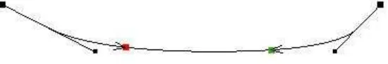
Spline Control Points
Spline control points are used in Flexsim when laying out a travel path network. Flexsim uses spline technology to give you a convenient method to add curves, inclines, and declines to NetworkNode paths.
These green boxes indicate the attributes of the path going in the indicated direction. Green means it is a passing path, yellow means it is a nonpassing path, and red means it is a "no connection" or in other words it is a one-way path going the other way. To switch between these colors, you can right click on the node and select an option. (Figure 3-3). You can also make the path a curved path by selecting the "Curved" option in the drop down menu. This will create two spline control points that you can move to create a curved path. You can also configure how connections are made by default using the Travel Networks Utility.
Spline Control Point parameters
Once you have created a curved path, move the small control points with the mouse.
NetworkNodes can be configured to specify the direction of the path. Again, you can use the right-click menu on the colored box, or, for a quicker method, you can hold down the "X" key and click on the colored box. (Figure 3-9).
Figure 3-9. Single direction path
When a path has been configured using spline paths, the travelers that use the path will automatically follow the spline that has been defined. The display of the spline control points, as well as the colored boxes, can be toggled on and off by holding down the "X" key and clicking on one of the NetworkNodes in the path network (Figure 3-10). Multiple "X" clicks will toggle between several different visual modes for the network.
The Model Tree View
The model tree view is used in Flexsim to explore the model structure and objects in detail.
The model tree view is a view window that provides many unique features. In this view you can:
Customize Flexsim objects using C++ or Flexscript
View all object data
Access the properties windows
Edit the model, delete objects, and modify all data
If you follow a few simple navigation rules you will find the tree view one of the most versatile views within Flexsim. The underlying data structure in Flexsim is contained in a tree. The many edit windows within Flexsim are simply graphical user interfaces (GUIs) that display filtered data from the tree. Since all tree views in Flexsim work the same way, once you understand how the tree view works you will be able to navigate and understand the structure of any tree view that is accessible.
Tree View Basics
Flexsim has been designed to hold all data and information in a tree structure. This tree structure is the core data structure for all of Flexsim's object oriented design. Those who are familiar with C++ object oriented programming will immediately recognize Flexsim's tree view as the C++ standard for object oriented data management.
There are several symbols used in the tree view that will help you understand the structure as you navigate the tree.
currently open windows. When a session is saved the MAIN tree and the VIEW tree are saved together.
The folder icon identifies a node that does not have any object data, but may contain other folders or objects.
The object icon is used to represent Flexsim objects in the tree view.
The node icon is used to specify data nodes within an object. Data nodes can have
additional data nodes placed inside them. If a data node has a "+" just to the left of the icon it will contain one or more additional data nodes. Data nodes can hold numeric or alphanumeric values.
Certain data nodes are used to hold executable code. There are four types of code nodes in Flexsim:
C++. C++ code must be compiled before running the model.
Flexscipt. This code will be auto-compiled during the running of the model. Read more details on writing logic in Flexsim.
Dll. This node refers to a Flexsim compatible pre-compiled dll. To create such a dll you would need to use a special Visual C++ project. This project is available on the user community.
Global C++. This is C++ code that is globally scoped. It must contain complete functions. These functions can be accessed by any node nested below this node. Typically this type of node is found as the first node under the main Tool folder.
When you select an object in the tree view by clicking on the icon with the mouse, the tree view will display the object as follows:
As objects and data nodes are expanded, the tree view can quickly grow to be outside the viewing limits of the tree view window. Flexsim allows you to move the tree around in the window by using the mouse. To move the tree around in the window just click-and-drag on the left side of the tree, use the mouse wheel to scroll up and down, or use the scroll bar on the side.
Data nodes can be expanded by clicking on the "+" to the left of the node icon. Since data nodes can have values or text you will see the text information or the data values to the right of the node.
As you can see, the tree is the repository of all data for the model. The properties windows are used to provide a more user-friendly way to manipulate the data in the tree. It is possible to completely edit your model from the tree, but it is recommended that you use the properties windows to avoid inadvertent deletion of model data. The properties windows are accessible in a tree view by double-clicking on the object icon or by selecting Properties from the right-click menu
Step-By-Step Model Construction
Building Model 3
To start building model 3, you will need to load model 2 from the last lesson.
If at any time you encounter difficulties while building this model, a fully functional tutorial model can be found at http://www.flexsim.com/tutorials
Step 1: Load Model 2
Load model 2 if it is not already open.
Step 2: Reconfigure the layout of Conveyors1 and Conveyor3
Now we are going to change the layout of the three conveyors so that they have a curved section at the end to convey the flowitems closer to ConveyorQueue. You might want to experiment with this Layout tab to create complex curves and rises. Have some fun!
Double-click Conveyor1 to open its Properties window.
Click the Layout tab. You can find more information about this page here.
Click Add to add a section of conveyor at the end.
Select Cureved from the Type list.
Edit the angle and radius values in the table so that Conveyor1 curves into the ConveyorQueue as shown below.
Step 3: Delete the sink
Highlight the Sink and press the Delete key.
When an object is deleted, all port connections to and from that object are deleted as well. Beware that this may affect the port numbering of those objects that were connected to the deleted object.
Step 4: Create three Racks
Create three Racks, place them to the right of ConveyorQueue, and name them Rack1, Rack2, and Rack3. Place the racks far enough away from the queue to allow the fork truck some travel distance to reach the racks.
Step 5: Create a Global Table to Control Flowitem Routing
The next step is to set up a global table that will be used to reference which rack each flowitem will be sent to (or more accurately stated, which output port of the conveyor queue the flowitems will be sent through). It is assumed that output port 1 was connected to Rack1, port 2 to Rack2, and port 3 to Rack3. If the connections are not in the correct order, you can modify them through the queue's properties window on the General tab in the Ports section.
We will send all itemtype 1s to Rack2, all itemtype 2s to Rack3, and all itemtype 3s to Rack1. Here are the steps to setting up a global table:
Change the Name to Rout.
Set Rows to 3 and Columns to 1.
Name the rows Item1, Item2 and Item3, then fill in the values which correspond to the output port number (rack number) we want to send the flowitems to.
Click the OK button to apply the changes and close the table.
You can learn more about global tables here.
Step 6: Adjusting the Send To Port Option on the ConveyorQueue
Double-click on ConveyorQueue to bring up its Properties window.
Click the Flow tab. Select the option By Global Table Lookup from the Send To Port list. The code template window will appear. Edit the blue text to read as follows:
Table: "Rout"
Row: getitemtype(item)
Column: 1
Click the OK button to close the Properties window.
Step 7: Reset, Save, and Run
Step 8: Adding NetworkNodes to develop a path for the Fork Truck
NetworkNode's are used to develop a path network for any task executer object, such as a Transporter, Operator, ASRSvehicle, Crane, etc. In the previous lessons we have used the operator and transporter to transport flowitems around the model. Up to this point we have let the task executer move freely across the model in a direct line between objects. Now we would like to confine the travel of the fork truck to a specific path as it transports flowitems from the conveyor queue to the racks. The following steps are used to set up a simple path.
Create NetworkNodes near the conveyor queue and each of the racks. Name them NN1, NN2, NN3, and NN4. The nodes will become the pick-up points and drop-off points in the model. You may add additional nodes between these nodes, but it is not necessary.
The last step is to connect the fork truck to the node network. In order for the fork truck to know that it has to use the path, it must be connected to one of the NetworkNodes in the path network. Connect the Transporter to NN1 (A key). This node now also becomes the starting point for the fork truck when you reset the model.
Step 9: Reset, save, and run the model
Now it would be a good idea to Reset, Save, and then Run the model to make sure the fork truck is using the network paths.
A word about offsets
Offsets are used by the fork truck to locate where the flowitem needs to be picked up or dropped off in the object. This allows the fork truck to travel into the queue and pick up the box, and travel to the specific cell in the rack to drop off the box. To force the fork truck to stay at the NetworkNode and not to travel off the path network, select "Do not travel offsets for load/unload tasks" from the drop down pick list found below the field entitled
Deceleration.
Step 10: Using reports to view output results
To view summary results of the simulation after having run the model for a period of time, select the main menu option Statistics > Reports and Statistics.
Go to the Summary Report tab of the Reports and Statistics dialog window.
Step 11: Running multiple runs of your model using the Experimenter
To access the Experimenter in Flexsim, select the main menu option Statistics > Experimenter.
The Simulation Experiment Control window will appear
The Simulation Experiment Control window is used to run multiple replications of a given model, and to run multiple scenarios of a model. When running multiple scenarios, you can declare a number of experiment variables, and then specify the values you want these variables to be set to for each of the scenarios you want to run. Confidence intervals are calculated and displayed for each of the performance measures you define on the Performance Measures tab. For more information on the experimenter, refer to the