Jin-Xin relaxation method used to solve the one-dimensional inviscid Burgers equation.

(1)

(2)

This content has been downloaded from IOPscience. Please scroll down to see the full text.

Download details:

IP Address: 202.94.83.93

This content was downloaded on 06/06/2017 at 09:44

Please note that terms and conditions apply.

View the table of contents for this issue, or go to the journal homepage for more

(3)

1

Content from this work may be used under the terms of theCreative Commons Attribution 3.0 licence. Any further distribution of this work must maintain attribution to the author(s) and the title of the work, journal citation and DOI.

Published under licence by IOP Publishing Ltd

1234567890

Conference on Theoretical Physics and Nonlinear Phenomena 2016 IOP Publishing IOP Conf. Series: Journal of Physics: Conf. Series 856_{(2017) 012007} _{doi :10.1088/1742-6596/856/1/012007}

Jin–Xin relaxation method used to solve the

one-dimensional inviscid Burgers equation

Sudi Mungkasi1

, Bernadeta Wuri Harini2

and Leo Hari Wiryanto3 1

Department of Mathematics, Faculty of Science and Technology, Sanata Dharma University, Mrican, Tromol Pos 29, Yogyakarta 55002, Indonesia

2

Department of Electrical Engineering, Faculty of Science and Technology, Sanata Dharma University, Mrican, Tromol Pos 29, Yogyakarta 55002, Indonesia

3

Department of Mathematics, Faculty of Mathematics and Natural Sciences, Bandung Institute of Technology, Jalan Ganesha 10, Bandung 40132, Indonesia

E-mail: [email protected], [email protected], [email protected]

Abstract. We consider the Burgers equation and seek for its numerical solutions. The relaxation method of Jin and Xin, called the Jin–Xin relaxation method, is tested to solve the Burgers equation. We find that the Jin–Xin relaxation method solves the Burgers equation successfully. In addition, the Jin–Xin relaxation method holds the analytical properties of the Burgers equation better than the standard Lax–Friedrichs finite-volume method does.

1. Introduction

Conservation laws govern a number of physical and mathematical problems. In physics,

they relate to transport of conserved quantities, such as mass, momentum and energy. In mathematics, they may occur as a constraint in optimal control problems and other optimization problems, for example, minimizing costs, maximizing revenue, etc.

Some previous works related to conservation laws are available in the literature. Conservation laws were successfully applied to simulate real world problems, such as floods and tsunamis as presented by Mungkasi and Darmawan [1]. Investigation on Adjoint IMEX-based schemes for control problems was conducted by Banda and Herty [2] using the relaxation method of Jin and Xin [3] (the Jin–Xin relaxation method). Yohana [4], as well as Yohana and Banda [5], extends the investigation to the Euler equations of gas dynamics employing the work of Armijo [6]. Even though the Jin–Xin relaxation method has been implemented successfully by Jin and Xin [3] themselves, as well as by the authors of [2,4,5], to solve some problems, to our knowledge, there is no publication testing the method to solve the one-dimensional inviscid Burgers equation.

In this paper we solve the one-dimensional inviscid Burgers equation using the Jin–Xin relaxation method. Note that the Burgers equation is a member of the class of conservation laws. Our work complements the aforementioned literature. We also solve the Burgers equation using the standard Lax-Friedrichs finite-volume method, as a benchmark, to compare the results with.

This paper is organized as follows. We write the problem formulation of the Jin–Xin

(4)

2

2. Problem formulation

In this section, we describe the problem that we want to deal with. We write the mathematical model under consideration first and the approach to solve the model afterward. We assume that the model is one-dimensional and scalar.

First, let us recall the general mathematical model that we want to solve. The general mathematical model governing the one-dimensional scalar conservation law is

ut+f(u)x = 0, (1)

for the time variable t_∈[0,_∞) and the space variable x_∈(_−∞,_∞) with the initial condition

u(x, t= 0) =u0(x). (2)

Here u = u(x, t) denotes the conserved quantity and f(u) represents the flux function. The functionu0 gives the initial condition of the conserved quantity. The conserved quantity can be mass, momentum or energy. Equation (1) is generally nonlinear. Note that, taking f(u) =1

2u 2_,

(1) becomes the one-dimensional inviscid Burgers equation [7].

Now, to solve (1) with the initial condition (2) let us recall the relaxation approach of Jin and Xin [3], that is, the Jin–Xin relaxation method. Jin and Xin [3] proposed that (1) and (2) be approximated by a relaxation system, which is a linear system of partial differential equations. The Jin–Xin relaxation system for the mathematical model (1) is [3]

ut+vx= 0, (3)

vt+aux =−

1

ǫ(v−f(u)), (4)

where the initial conditions relating to (2) are

u(x,0) =u0(x), (5)

v(x,0) =f(u0(x)). (6)

Here v=v(x, t) is a dummy variable andais a positive constant satisfying

−√a_≤f′₍_u₎_≤√_{a ,} ₍₇₎

for all u. The parameter ǫ is positive and called the relaxation rate. When the solution is smooth, we eliminate variable v from (3) and (4) to obtain

ut+f(u)x=ǫ(auxx−utt). (8)

Forǫ_→0+_{, we observe that (8) tends to (1). That is, for}_ǫ

(5)

3

1234567890

3. Numerical method

We write the numerical scheme to solve (3) and (4), that is, the relaxation system of (1). Let us assume that the space and time domains are discretized in the finite volume framework. The space domain is discretized uniformly with the cell width h. (Readers interested in nonuniform space discretization can consult the work of Mungkasi [8].) The time domain is discretized uniformly with the time step k. The notation un_j is for pointing the approximate value of u in thej-th cell at the n-th time step.

In this paper we use the upwind numerical technique as follows [3]. Discretizing (3) and (4) with respect to space and time domains, we obtain the one-step conservative explicit scheme:

un_j+1₋un_j derived the first-order upwind relaxing fluxes, which are given by

un_j+1/2=

Using the upwind fluxes (11) and (12) in the one-step conservative explicit schemes (9) and (10) we obtain the upwind numerical method for (3) and (4) as

un_j+1₋un_j

Therefore, given that we know the quantities un_j and vn_j at the n-th time step for all j cells, using (13) and (14) we can compute the quantities and at the (n+ 1)-th time step for allj cells. This can be done by iterations. Starting from the initial condition (2), we have (5), so we obtain u0

j. We also have (6), so we obtain v0j. Then the values of u1j,vj1,uj2, v2j, u3j, v3j,... are also obtained for all j using (13) and (14).

4. Numerical results

In this section we present results of our research. The Jin–Xin relaxation method is applied to solve the inviscid Burgers equation. The results of this method are analyzed if they hold some analytical properties of the Burgers equation. We also compare the results of the Jin–Xin relaxation method to those of the standard Lax-Friedrichs finite-volume method to show that the Jin–Xin relaxation method performs better. All quantities are assumed to be in the SI units, so we do not need to write their units.

As we have mentioned in Section 2, let us take f(u) = 1 2u

2

(6)

4

0 2 4 6 8 10

0 0.5 1 1.5 2

x

u(x,t)

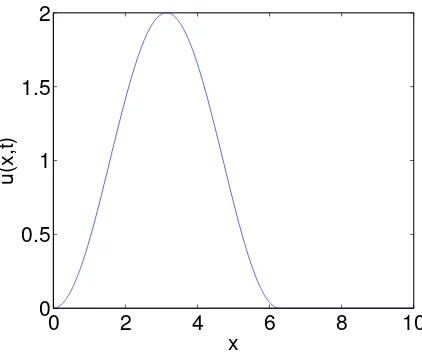
Figure 1. Initial condition for the Burgers equation at timet= 0.

For simulations, we set up the followings. We consider the space domain 0_≤ x _≤10. The initial condition is given by

u0(x) =

  

 

1₋cosx, if 0< x_≤2π,

0, if 2π < x_≤10.

(16)

The boundary condition is

u(0, t) =u(10, t) = 0 (17)

for all t > 0. For all simulations, we take the cell width to be h = 10−2 _{and the time step to} be k= 10−3

. This time-step value is chosen so, in order that methods are stable. The Jin–Xin relaxation rate is taken as ǫ= 10−3_.

Let us collect some analytical properties of our simulation setting. With the initial condition

given by (16), the maximum height of the wave is 2, as shown in figure 1. Due to the

characteristics of the Burgers equation, the wave propagates from the left to the right direction. Based on the formulation of LeVeque [9], the wave will form a shock discontinuity starting at timets=−1/min{u′0(x)}, that is,ts= 1. Therefore, a shock wave will propagate from the left to the right at time t > 1. When the shock occurs, the wave loses some energy, so the wave height gets smaller over time. Using these properties, we shall analyze our numerical results.

Representations of Jin–Xin relaxation results are shown in figure 2. From our simulation, we observe that the wave height is kept at the value of 2 until time ts= 1, as given in figure 2(a). Then for timet >1, a shock occurs and the wave height gets smaller than 2. We also notice that the shock is sharply resolved by the Jin–Xin relaxation method, as illustrated in figure 2(b).

(7)

5

1234567890

0 2 4 6 8 10

Figure 2. Solutions to the Burgers equation using the Jin–Xin relaxation method.

0 2 4 6 8 10

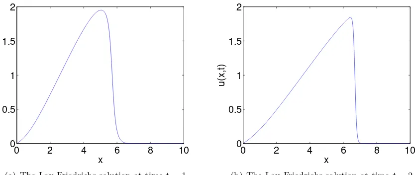
(a) The Lax-Friedrichs solution at timet_{= 1.}

0 2 4 6 8 10

(b) The Lax-Friedrichs solution at timet_{= 2.}

Figure 3. Solutions to the Burgers equation using the Lax-Friedrichs finite-volume method.

We can now compare the results of the Jin–Xin relaxation method and those of the Lax-Friedrichs finite-volume method. Comparing figure 2(a) and figure 3(a), we obtain that the Jin–Xin relaxation method holds the analytical property of the wave height better than the Lax-Friedrichs finite-volume method does. Furthermore, comparing figure 2(b) and figure 3(b), we notice that the Jin–Xin relaxation method holds the analytical property of the shock discontinuity better than the Lax-Friedrichs finite-volume method does.

5. Conclusion

(8)

6

Acknowledgments

This work was financially supported by Sanata Dharma University and a research grant from

Direktorat Riset dan Pengabdian Masyarakat (DRPM) of Ministry of Research, Technology and Higher Education of the Republic of Indonesia year 2016.

References

[1] Mungkasi S and Darmawan J B B 2015 Proc. 4th Int. Conf. on Soft Computing, Intelligent System and Information Technology (Bali)vol 516 ed Intan Ret al(Springer-Verlag) p 469

[2] Banda M K and Herty M 2012Comput. Optim. Appl.51909 [3] Jin S and Xin Z 1995Commun. Pure Appl. Math. 48235

[4] Yohana E 2012 MSc Thesis University of the Witwatersrand at Johannesburg [5] Yohana E M and Banda M K 2016J. Numer. Math.2445

[6] Armijo L 1966Pac. J. Math.16₁

[7] Mungkasi S 2015IOP Conf. Ser.: Mater. Sci. Eng.78012031 [8] Mungkasi S 2016Adv. Math. Phys.2016_7528625

[9] LeVeque R J 1992Numerical Methods for Conservation Laws(Basel: Springer)