receptor deep sequencing data
Duncan K. Ralph1,*, Frederick A. Matsen IV1
1 Fred Hutch, Seattle, Washington, USA
ABSTRACT
The collection of immunoglobulin genes in an individual’s germline, which gives rise to B cell receptors via recombination, is known to vary significantly across individuals. In humans, for example, each individual has only a frac-tion of the several hundred known V alleles. Furthermore, this set of known V alleles is both incomplete (particularly for non-European samples), and con-tains a significant number of spurious alleles. The resulting uncertainty as to which immunoglobulin alleles are present in any given sample results in inac-curate B cell receptor sequence annotations, and in particular inacinac-curate inferred naive ancestors. In this paper we first show that the currently widespread prac-tice of aligning each sequence to its closest match in the full set of IMGT alle-les results in a very large number of spurious allealle-les that are not in the sam-ple’s true set of germline V alleles. We then describe a new method for infer-ring each individual’s germline gene set from deep sequencing data, and show that it improves upon existing methods by making a detailed comparison on a variety of simulated and real data samples. This new method has been inte-grated into the partis annotation and clonal family inference package, available athttps://github.com/psathyrella/partis, and is run by default with-out affecting overall run time.
AUTHORSUMMARY
Antibodies are an important component of the adaptive immune system, which itself determines our response to both pathogens and vaccines. They are produced by B cells through somatic recombination of germline DNA, which results in a vast diversity of antigen binding affinities across the B cell repertoire. We typi-cally learn about the development of this repertoire, and its history of interaction with antigens, by sequencing large numbers of the DNA sequences from which antibodies are derived. In order to understand such data, it is necessary to deter-mine the combination of germline V, D, and J genes that was rearranged to form each such B cell receptor sequence. This is difficult, however, because the im-munoglobulin locus exhibits an extraordinary level of diversity across individuals – encompassing both allelic variation and gene duplication, deletion, and conver-sion – and because the locus’s large size and repetitive structure make germline sequencing very difficult. In this paper we describe a new computational method that avoids this difficulty by inferring each individual’s set of immunoglobulin germline genes directly from expressed B cell receptor sequence data.
1
INTRODUCTION
The heavy and light chain B cell receptor (BCR) loci arise from a random re-combination of germline V, D, and J genes. Repeated across many B cells, this generates the vast diversity of naive BCRs that is integral to the adaptive immune system. As an additional source of population-wide variation, there is significant variation of germline genes between individuals. Databases such as IMGT [1] aim to collect and organize this ensemble of germline genes.
The analysis of BCR sequence data begins with the alignment of each sequence against a set of germline V, D, and J genes. A variety of methods (e.g. [2–5]) have been developed to accomplish the basic task of deciding which V, D, and J genes gave rise to each observed sequence. There has been less work, however, toward measuring the extent to which the set of germline genes used for this analysis resembles the germline gene set actually present in the individual from which the sequence data was derived. Most methods simply use the full set of germline genes from a database such as IMGT [1] for all samples.
One problem with this approach is that the IMGT set includes genes from all individuals of a species, while any single individual’s germline contains only a fraction of these (roughly 50 out of 250 V genes, 25 of 35 D, and 6 of 12 J). This is problematic for sequencing studies that use antigen-experienced B cells that have been through several rounds of somatic hypermutation (SHM), which obscures the identity of the original germline gene. As we show below, this leads to large numbers of spurious gene assignments, and an inferred germline gene set with many more alleles than are in the individual’s true set.
Another problem with this approach is that no database contains a perfect cat-alog of the complete immunoglobulin germline diversity of each species. Se-quencing continues to uncover novel human V genes that are not in any previous database [6–13]. Additionally, a significant fraction of the sequences in existing databases are likely the result of sequencing error rather than real biological vari-ation [14–16]. Our knowledge of the immunoglobulin locus is even less complete for other species [12, 17].
Improving our understanding of the immunoglobulin locus, however, is not simply a matter of applying standard genome sequencing protocols more broadly. Most genome sequencing is performed on lymphoblastoid cell lines [18–20], whose prior rearrangement has destroyed much of the information about the original im-munoglobulin locus. The obvious solution would be to sequence other cell types; however assembly challenges due to the complexity and repetitiveness of the lo-cus [21] mean that even sequencing an intact immunoglobulin lolo-cus is not straight-forward. The IGHV locus, for instance, consists of about 120 V genes, roughly two-thirds of which are non-functional pseudogenes, spread over a megabase of chromosome 14 [9]. The immunoglobulin locus is also subject to widespread gene duplication, deletion, and conversion [7, 8, 22, 23]. Thus although databases such as the 1000 Genomes project and the Simons Genome Diversity Project can be used to investigate immunoglobulin diversity [23, 24], this approach is not without pit-falls [25].
would impact, for example, recent work on the effects of the presence or ab-sence of individual alleles on broadly neutralizing anti-influenza antibody devel-opment [26]. Second, such misassignment leads to inaccurate inferred naive an-cestor sequences. Efforts to synthesize these inaccurate ancestral sequences in the lab and study their binding properties may then result in erroneous conclusions, since even single amino acid changes can have large effects on affinity [27]. And finally, studies of mutation [28, 29] and selection [30, 31] during affinity matura-tion depend upon accurate inferred naive sequences in order to correctly identify somatic mutations.
Our current understanding of the immunoglobulin locus comes largely from a small number of low-throughput genome and BAC library sequencing studies. The first complete sequence of the locus [32], which has been included in the first few drafts of the human genome, was assembled from several different cell lines and is therefore not a haplotype. More recently, a single complete haplotype of the heavy [9] and light [10] chain loci has been published. In addition to these larger efforts, many less-comprehensive studies of the locus have been cataloged atwww.imgt.org.
Advances in sequencing technology, however, have allowed progress to come also from inference on expressed BCR repertoires. Several initial studies inferred germline sets by combining computational analysis with expert scrutiny, with one paper reporting a high level of diversity with many novel (non-IMGT) alle-les across 12 individuals [7], and a second extending those results to 18 complete haplotypes [8]. Similar work by a different team used naive sequences to infer germline sets and haplotype linkage information for two individuals [33]. None of these studies, however, resulted in a generally-applicable software package or included a broad-scale validation of their methods.
More recently, software packages have been developed that enable fully-automated germline inference including novel allele discovery. TIgGER [11] uses a detailed per-position fitting procedure to find new alleles separated by a small number of point mutations from genes in a known database, and a heuristic prevalence threshold-based procedure to infer germline sets. The IgDiscover package [12] infers germline sets using Levenshtein distance-based hierarchical UPGMA clus-tering on low-SHM IgM samples. This approach allows IgDiscover to find new al-leles separated by an arbitrary number of point mutations and insertion/deletion events, and frees it from the need for an initial species-specific starting database.
elevated levels of SHM, it is more generally applicable than IgDiscover, which is restricted to low-SHM IgM samples. In addition, while TIgGER and IgDiscover are essentially standalone germline set inference packages, our method is inte-grated with and run by default in the general-purpose partis package, which also provides simulation, annotation, and clonal family inference. Because D inference would be very challenging, and because the J locus varies much less between indi-viduals than either V or D, in this paper we follow these other software packages in limiting ourselves to studies of V diversity.
Because of the high prevalence of both single nucleotide polymorphisms (SNPs) and structural variants in the immunoglobulin locus, there is no single reference genome to which all variants can be mapped, and thus standard SNP nomencla-ture appears insufficient. In this paper the usage of “gene” and “allele” is thus largely interchangeable. In addition, we define the “germline haplotype” as the set of germline genes on a single chromosome, while “germline gene set” refers to the full set on both the maternal and paternal chromosomes. In cases where confusion is unlikely, the latter will be shortened to “germline set”.
RESULTS
Simulation methods summary. In order to establish an expectation for how germline inference methods will perform on real data, we first investigate performance on a number of simulation samples. BCR repertoires differ significantly in many differ-ent variables such as SHM levels, germline set complexity, and clonal family struc-ture. Although we would in principle like to explore germline inference accuracy by varying all of these variables simultaneously, this is combinatorially infeasible, and we thus adopt a two-stage approach to validation. We first vary one vari-able at a time, while holding all others constant, using simplified “sparse” reper-toires consisting of sequences stemming from only a few genes. We then choose several representative values for each variable, and simulate full, realistic reper-toires at these values. Geometrically, this can be imagined as investigating perfor-mance first along many slices through the parameter space, and then at several fixed points. This approach is motivated by the fact that, in sequence-similarity space, realistic repertoires are composed of widely-spaced groups of genes, where each group consists of a few genes that are much closer to each other than the typical between-group spacing. The genes within each group are thus easily con-fused with each other due to SHM, but not with genes in other groups. The sparse repertoires effectively recreate the dynamics within such a group, while allowing exploration of a much larger portion of parameter space than if we were to use full repertoires for all simulations.
In this paper, the germline set for each sparse repertoire consists of one known germline gene, and either one or two novel alleles. Each full-repertoire sample, meanwhile, is generated by choosing a number of V, D, and J genes, and some number of alleles for each of these genes, based on results from germline sequenc-ing studies (see Methods), which results in roughly 55 V, 25 D, and 6 J alleles per sample.
FIGURE1. Fraction of true alleles missing(not inferred) by par-tis on simplified “sparse” repertoires for a variety of variables as a function of the number of sequences in the sample. Top left:SHM levels (the SHM distributions corresponding to “low”, “typical”, and “high” are shown in Fig S1).Top right:new-allele prevalence (as a fraction of the existing allele’s prevalence). Mid-dle left:number of SNPs (Nsnp) separating new and existing
alle-les. Middle right:Nsnpwith multiple new alleles, where, e.g. “1
+ 3” indicates two new alleles, separated by 1 and 3 SNPs from the same existing allele. Bottom left:mean number of leaves per clonal family. Bottom right: tree balance. Each point represents the mean performance (±standard error) on 50 independent sim-ulation samples of the indicated sample size.
FIGURE 2. Fraction of partis-inferred alleles not in the true germline set on simplified “sparse” repertoires for a variety of variables as a function of the number of sequences in the sample. For explanation see Fig 1.
repertoire that are missing from the inferred repertoire (Fig 1), and the fraction of spuriously-inferred alleles (that are not in the true repertoire, Fig 2) as a function of sample size for each variable.
Increasing the rate of SHM makes inference more challenging (Figs 1 and 2, top left, with the corresponding SHM distributions in Fig S1). Because allele infer-ence sensitivity is determined mainly by sequinfer-ences with a small number of SHMs (specifically, a number comparable to the number of SNPs separating the new and existing alleles), raising SHM rates effectively reduces sample size.
V naive inaccuracy # missing # spurious # correct
TABLE1. Summary full-repertoire simulation performance for the three germline inference methods plus “full IMGT” annota-tion. Results are the mean (±standard error) of ten independent 50,000-sequence samples for both low-SHM (top) and high-SHM (bottom).V naive inaccuracyis the mean Hamming distance be-tween true and inferred V region naive sequences (excluding the three most 3’ bases). We also show the mean number of true alle-les missing from the inferred germline set (# missing), the number inferred that are not in the true germline set (# spurious), and the number in common between the inferred and true germline sets (# correct). We show IgDiscover only for the low-SHM samples, since it is designed only for IgM.
The number of SNPs (Nsnp) separating a new allele from its most similar known
counterpart also affects the details of germline inference. We show performance for differentNsnpfor both a single new allele (Figs 1 and 2, middle left) and for
sev-eral combinations of multiple new alleles (Figs 1 and 2, middle right). Sensitivity is independent ofNsnpfor smallerNsnp(three or less), and then decreases slightly
with increasingNsnp. The presence of multiple new alleles, on the other hand,
does not appreciably affect sensitivity as long as their SNPs do not occur at the same positions. Because the occurrence of multiple new alleles with the same SNP positions is rare in real data, we do not show results for this case. In many cases it is in fact possible to disentangle such alleles, but this depends on the details of each new allele’s prevalence andNsnp.
The shared mutations within a clonal family complicate allele inference be-cause independent mutations are required for accurate fitting. We find that in-creasing clonality effectively decreases sample size (Figs 1 and 2, bottom left), rather than introducing the spurious alleles that would result from fitting with non-independent mutations. This indicates that our method of selecting a small number of sequences to represent each clonal family (see Methods) provides a sufficiently accurate method of choosing sequences with independent mutations.
We find that variations in phylogenetic tree shape do not greatly affect our method (Figs 1 and 2, bottom right). We change tree shape by using the TreeS-imGM package [38] to vary the shape parameter of a Weibull distribution control-ling an age-dependent speciation process.
FIGURE 3. Full-repertoire V naive accuracy (Hamming dis-tance between true and inferred V naive sequences) for the three germline inference methods, plus annotation with the full IMGT set. Each point represents the number of sequences (y) with a given error (Hamming distance, x). Shown on the first three repli-cates (0-2) of both the low-SHM (left), and high-SHM (right) full-repertoire simulation samples (see text).
these sparse samples because both methods use hard-coded assumptions tailored to typical full repertoires that cause crashes on these sparse repertoires.
We split these full-repertoire samples among two difficulty levels: ten samples with more-uniform allele prevalence and low SHM, and ten samples with less-uniform allele prevalence and higher, typical SHM (details in Methods). Results with IgDiscover are shown only for the low-SHM samples, since IgDiscover is designed to work only on low-SHM IgM-specific data.
We measure the influence of germline set accuracy on practical results in two ways: in terms of the actual genes and alleles inferred, and in terms of the result-ing annotation accuracy. The former is more relevant to germline databases and studies of gene association, while the latter is of more concern when inferring and studying the function of ancestral sequences.
We find that the practice of aligning against the full IMGT set results in a very large number of spurious gene inferences, even on low-SHM samples (Table 1 and Fig 4). The three explicit germline inference methods, while all giving much smaller numbers of spurious genes, harbor significant differences. The partis-inferred missing and spurious alleles are found on relatively short branches com-pared to those of the other programs (Figs 5, 6, 7). This results in partis’s signifi-cantly more accurate V naive inference (Table 1). By considering the distribution of Hamming distances between true and inferred naive V sequences (Fig 3), we see that the relative inaccuracy of TIgGER and IgDiscover is driven by rare se-quences that are assigned to genes that are very dissimilar to their true gene. We also note that TIgGER shows reduced sensitivity at typical SHM rates (Fig 6 right), compared to low SHM rates (Fig 6 left), in fact failing to infer any of the novel (non-IMGT) alleles at typical SHM rates.
These simulation samples, together with true and inferred germline sets, are available athttps://zenodo.org/record/1037464#.WfISc3BrwUE.
Results on real data. In order to evaluate performance on real data, it would be natural to deep sequence individuals for whom we also have accurate results from germline sequencing. Unfortunately, as described above, the difficulty of germline sequencing means that such samples are not readily available. We instead use two types of comparison that, while not definitive, provide some insight.
We first compare results from the different inference methods when run on the same sample, and find agreement on 70-90% of the total genes (Figs 8, 9, 10, S2, S3). While this is reassuring, some caution is advised, as the methods are far from uncorrelated (see Supplement). IgDiscover is shown only for IgM samples (Fig 10, and non-IgM samples with very low SHM rates (Figs 8, S2, S3). Also of note is the large cluster of closely-related novel alleles inferred only by TIgGER in the IgM data from subject lp23810 [36] (Figs 10, 13).
We next compare the results of each inference method on several different sam-ples from the same individual. We find a similar overall level of agreement both when comparing samples from different time points (Figs 11, 12), and of different isotypes (Fig 13). These comparisons give some idea of each method’s uncertainty because, while the physical germline genes are in each case identical, the SHM rates, gene expression levels, and clonal family structure vary significantly with both time and isotype.
for a single haplotype, while another [39] reported a range of 38-46 per haplotype. In order to convert these per-haplotype totals to per-diplotype totals, we calculate the mean fraction of alleles shared between the inferred germline sets from two unrelated individuals. For the sequencing data in this paper, this mean overlap is 67% (range 50-85%). This suggests that to go from per-haplotype to per-diplotype totals we multiply by1 + (1−0.67), which yields per-diplotype estimates of 57 for [9] and 51-61 for [39]. These values, both for total genes and for the fraction of genes shared between unrelated parental haplotypes, roughly agree with two other studies that found 35-46 per haplotype and 39-55 per diplotype [8], and 45-60 per diplotype with a mean alleles per gene of 1.2 [7]. The mean total number of partis-inferred V genes observed in individuals in this paper, meanwhile, is 47 (range 38-62). This suggests that the sample sizes, clonal family structures, mu-tation rates, and expression levels, together with our method’s sensitivity, result in a failure to detect about 0 to 10 genes per individual. We have not accounted for spuriously-inferred alleles in this calculation because our validation results suggest that when partis does infer spurious alleles, each simply replaces a very similar true allele, and thus does not have an appreciable net effect.
The fasta files for each inferred germline set are available athttps://zenodo. org/record/1037464#.WfISc3BrwUE. We have made the command-line script used to make phylogenetic comparison plots available for general application at https://git.io/vFo2B.
DISCUSSION
We have developed a practical new tool for inferring per-sample immunoglobu-lin germimmunoglobu-line gene sets, and performed extensive validation and comparison against existing tools. Our tool is implemented in the existing partis annotation and clonal family inference package. We have shown, first, that the currently widespread practice of aligning expressed BCR samples against the full IMGT germline set results in both large numbers of spurious alleles and inaccurately inferred naive ancestors. Second, we showed that our method infers significantly more accurate germline sets than the existing TIgGER and IgDiscover methods in terms of both inferred gene similarity and naive ancestor inference, but of similar accuracy in terms of raw number of genes. We also showed that so far as we can determine using a wide variety of comparisons, our method’s performance on real data is similar to that on simulation.
(roughly a few thousand sequences or less). Also, we have thus far only applied our method to V region genes, although the extension to D and J should be concep-tually straightforward. Finally, taking advantage of the fact that rearrangement occurs only between genes on the same chromosome, as in [8, 33], would likely provide additional improvement.
A further limitation of our method is that it looks only for new alleles separated by SNPs from existing alleles, and not for those separated by insertion/deletion events. While this is not a significant limitation on human samples, the IMGT germline sets for other species are incomplete enough that, in those species, this could cause novel alleles to be misinterpreted as SHM indels. This is one respect in which the clustering-based approach taken by IgDiscover offers a significant advantage (see Supplement). For this reason we have also implemented a non-default clustering-based method which can be run in addition to the purely muta-tion accumulamuta-tion plot-based method described here (see Manual). While we thus recommend this clustering-based method for non-human samples, its robustness, like IgDiscover’s, can suffer on some highly-mutated samples, so we have left it as a non-default option pending future improvements.
METHODS
Overview. The task of inferring germline genes consists largely of learning to dis-tinguish between positions that are highly mutated as a result of SHM, and those whose highly-mutated appearance stems from the occurrence of previously un-known alleles. A few key observations allow us to extract enough information to make this distinction. First, in the absence of unknown alleles, the probability of a mutation at each position in an observed sequence is roughly proportional to the total number of mutations in that sequence (at least at the low SHM levels relevant for new-allele inference). In other words, while mutation rates differ dramatically from position to position according to, for instance, hot and cold spot motifs, each position is more likely to be mutated in sequences that have been subject to higher levels of SHM. In the presence of unknown alleles, on the other hand, sequences stemming from these unknown alleles will be mistakenly assigned to the most similar known allele, causing this approximate proportionality to be violated. If there are, say,NsnpSNPs separating a known and unknown allele, then there will
be very few sequences from this unknown allele that appear to have fewer than
Nsnpmutations. TheNsnppositions at which they differ, on the other hand, will
almost always appear to be mutated in sequences that appear to containNsnpor
more total mutations. This differing apparent mutational behavior between se-quences with fewer than, as compared to more than,Nsnpmutations provides the
basis for our method.
and then follow the procedure above for each such group. We first show exam-ple plots for three simexam-ple, hypothetical repertoires (Fig 14). While these simexam-ple repertoires, by themselves, are gross simplifications of the biological complexity in a real BCR repertoire, they contain the essential elements from which we can construct a method that performs well on real data sets.
Models and fitting. In the context of mutation accumulation plots (Fig 14), the presence of new alleles is signaled by a departure from what would be expected if all sequences had been assigned to the correct true gene. Namely, to the extent that mutations at each site accumulate in proportion to the total number of mutations in the sequence, correct assignment would result in simple linearity. For incorrect assignment, this linearity is replaced with differing behavior between the regions below and aboveNsnp. Our task, then, amounts to distinguishing between plots
that can be adequately described by a one-piece linear model, and those that re-quire a model consisting of two pieces separated by a discontinuity.
In order to distinguish these two hypotheses, we construct a model for each. The one-piece model is simply a linear fit constrained to pass through the origin. The two-piece model, meanwhile, consists of two separate linear fits, which we call the “lower” (belowNsnp) and “upper” (aboveNsnp) fits. The lower fit is
con-strained to pass through the origin, while the upper fit’s y-intercept must be near the average of the upper-region mutation frequencies (within 1.5 standard devi-ations of their mean). The junction between the two pieces must harbor a signif-icant discontinuity in either bin value (mutation frequency) or bin total (number of sequences per bin), where significance is defined as a difference of more than 2.5 times the larger uncertainty. This two-piece model describes the presence of a new allele separated by Nsnp SNPs from the original known gene. To give a
general idea of the implementation, several examples are shown in Fig 15. We use a ratio of error descriptors to determine whether a plot is adequately described by the one-piece fit. Defineǫto be the sum of squared residuals divided by degrees of freedom, which in regression analysis is sometimes called the mean squared error. Good fits are characterized by values ofǫaround one, while val-ues much greater than one indicate poor fits. Valval-ues significantly less than one generally indicate poorly-estimated uncertainties. For our purposes, then, we are interested in positions (which we call “candidate positions”) for whichǫis large for the one-piece fit (greater than 4.5) but around one (less than 1.95) for the two-piece fit.
For eachNsnp, we construct the most plausible potential new allele by finding
theNsnppositions that have the worst one-piece, but best two-piece, fits. We
quan-tify this using the ratio of the twoǫ,
(1) r= ǫ1-piece
ǫ2-piece
.
Because cases that would be better described by more complex models will have larger residuals (poor fits) for both one-piece and two-piece models, which cancel out in the ratio, this formulation provides robustness to deviations from linearity. The model for the best potential new allele consists of theNsnppositions that have
the largest values ofr.
size from many surrounding bins, we perform all fits in a window of width 10 bins. This window begins at zero for smallNsnp, while for largerNsnpit is symmetric
aroundNsnp.
We apply several additional criteria to ensure that the candidate fits make a compelling case for a new allele. The slope at the discontinuity, i.e. the slope de-fined by the two points on either side, must be much larger than both the upper and lower fitted slopes (a fractional difference of more than 2.5 times). For larger
Nsnp(five or more), the slopes before and after the discontinuity must also either
be consistent, or the lower slope must be the smaller of the two.
The unfortunate profusion of constant values in the preceding paragraphs de-serves some examination. In general, for the sake of simplicity and interpretability, we have wherever possible minimized the number of such constants. However, practical constraints make it difficult to reduce their number further. In theory, it would be possible to construct a more complicated model that faithfully recreated all the details of the real system, which would enable a collection of simple like-lihood ratio tests. However, in practice this approach is unlikely to be computa-tionally feasible, and would likely require a much lengthier development process. Instead, we have adopted the approach of comprehensively validating a simpler model which, nevertheless, provides an adequate description of the system’s real biological complexity. This method’s robust performance across a wide variety of data and simulation samples during this validation (only a small fraction of which appear in this paper) gives us great confidence in its general applicability.
Comparing multiple hypotheses. The previous section outlines a procedure for identifying a single potential new allele for each individualNsnp. In realistic
sam-ples, however, we must treat the general case where there may be several new alleles, either with the sameNsnp, or spread among severalNsnp.
To do this, we first sort every candidate position within eachNsnpby decreasing
r. In order to better adjudicate between ties in the first sort, we then sort again either by decreasing y-intercept (ifNsnpless than three) or decreasing two-piece fit
ǫ. The firstNsnpelements of this sorted list of candidate positions are then taken as
a candidate allele, the nextNsnppositions are taken as a second candidate allele,
and so on, until fewer thanNsnpremain. The second sorting step serves to group
together positions with similar fit properties, and that are thus most likely to come from the same new allele. These fit properties are affected by several aspects of the new alleles, most notably their prevalence. In cases with two new alleles with the same prevalence, for example, this is not an effective means of determining which positions go with which allele; however, in real data such cases are very rare.
For each of these candidate alleles, both the smallestramong their positions, and the mean, must be greater than 2.75. The discontinuities for every pair of positions must also be compatible, defined as the difference in bin totals (number of sequences) on either side of Nsnp, which must be closer than three times the
maximum of their two uncertainties.
This procedure is repeated for eachNsnp, resulting in a list of candidate alleles
from each; these lists are then merged into a final list that is sorted by decreasing
Nsnp. We then go through this list and discard alleles that share any positions with
Approximations and pre-filters. The procedure described above would work well in principle, but would require a computationally prohibitive number of fits. As a rough estimate, taking 50 initial, known alleles in a sample, each with 300 posi-tions, looking up throughNsnpequals eight, and with both the one-piece and
two-piece fits, we would need 360,000 individual linear fits. To be useful, however, it must run as part of the overall partis annotation, which takes only minutes on samples with tens of thousands of sequences. Luckily, the overwhelming majority of these fits can be avoided by ignoring uninteresting positions using a number of approximation procedures. The cumulative effect of the following approxima-tions and filters is that a typical run requires of order 100 fits, with no appreciable decrease in precision or sensitivity. This results in a method that does not add significant run time to an existing partis run.
The first step is to ignore positions for which there would not be enough sta-tistical power to have any sensitivity to new alleles. We thus skip positions with fewer than 150 total observed sequences, summed over bins. Positions with fewer than 30 observed mutations, also summed over bins, are similarly skipped.
For eachNsnp, we also ignore positions that do not have at least eight observed
mutations in theNsnpth bin. This bin is of primary importance, because it is the
means by which we determine that thisNsnpis the correct one, rather than those
slightly larger or smaller. If this bin is truly signaling a new allele, then it must contain a significant number of mutated sequences.
For several of the subsequent steps, we use an approximate fitting procedure to arrive at a slope, intercept, and associated uncertainties. While less accurate, and more heuristic, than the least-squares fits that are used elsewhere, it is also much faster. We begin by calculating the two-point slope between each pair of adjacent points. If there are only two points in total, this is supplemented by a “synthetic” slope between the first point shifted up, and the second shifted down, by their respective uncertainties. The approximate slope is then calculated as the mean of these pairwise slopes, with its uncertainty the associated standard error. We arrive at the approximate y-intercept with a similar procedure, except that the pairwise slope is replaced by the pairwise y-intercept, which uses the previously-calculated pairwise slope.
For smallerNsnp (three or less), we also require that the approximate
upper-region y-intercept fit bounds do not include zero. If they do include zero, there will not be a significant difference between the one- and two-piece fits. As an addi-tional, and more stringent, test that the upper-region y-intercept for these smaller
Nsnp is well above zero, we require that the approximate fit’s y-intercept is also
greater than zero.
ForNsnpequals two, we also require that the bin immediately before theNsnpth
bin be outside of the upper-region y-intercept fit bounds.
And finally, for largerNsnp(five or greater), the approximate lower fit’s slope
must be less than that of the approximate upper fit, in cases in which they are inconsistent.
The presence of incomplete V sequences clearly reduces our sensitivity to new al-leles simple by reducing the sample size for positions at each end. A more serious problem, however, is that differing lengths cause sequences to be assigned to in-correct bins, since their apparent number of mutations is different than their true number. In order to avoid this problem, we ensure that all analyzed sequences be-gin and end at the same aligned germline bases. To accomplish this, for each end (5’ and 3’), we find the deletion length such that only a small fraction (f, by de-fault 0.01) of sequences have a longer deletion length. We then exclude the fraction
f of sequences that have longer deletions. Among the remaining sequences, we then exclude from the analysis the positions that fall within these deletion lengths. For example, if 99% of sequences have 3’ deletions of four or fewer bases, then we would discard sequences with more than four 3’-deleted bases, and would not use that gene’s four most-3’ positions in the fitting procedure. Note that on the 3’ side of V, this exclusion procedure is especially important because the final few germline-aligned positions next to any non-templated insertion always have very poorly-measured mutation frequencies.
Collapsing clones. Our method requires that we consider only independent mu-tation events, excluding any mumu-tations that share a common ancestry. In order to satisfy this requirement we attempt to select from each clone the largest possi-ble set of sequences without shared mutations. In doing this, we give preference to relatively unmutated sequences, since most new alleles are separated by only a few SNPs from known alleles. Specifically, we sort the sequences from each clonal family in order of increasing apparent V mutation. We then traverse this list, selecting each sequence that does not share any mutations with a previously-selected sequence. As shown in [40] it would be straightforward to use the full partis method to separate the sequences into clonal families. However, for the pur-poses of ensuring independent mutations, there is little benefit to having precisely accurate clusters, since a slightly inaccurate clustering only results in slightly in-accurate uncertainties in the fits, and uncertainties on uncertainties are in practice never large enough to impact the analysis. For the sake of speed, then, we simply cluster using inferred naive sequences, i.e. every sequence that is inferred to have the same naive sequence is clustered together. This has the additional benefit of becoming more conservative as the sample size becomes large – in other words it tends to over-cluster more as the space of potential naive rearrangements fills up, and nearby rearrangement events have very similar naive sequences. This has the effect of sacrificing some sensitivity in order to ensure that mutations are actually independent.
Initial removal of less-likely alleles. Some care is necessary when constructing each sample’s initial set of known genes. We find the performance of our new-allele inference to be robust enough that the best approach is to first choose a min-imal number of genes whose presence in the sample is supported by very strong evidence. We then apply the new-allele inference framework in order to reinstate alleles for which the evidence was less overwhelming, along with any novel alle-les.
this partitioning cannot be accomplished using only the IMGT names – there are many cases of allelic variants that differ by so many SNPs that confusion is very unlikely, as well as alleles of separate genes that differ by only a single SNP. We construct these groups by single-linkage clustering such that genes with the same conserved cysteine position, and separated by fewer than eight SNPs, are grouped together. In order to ensure that we can re-infer all of the genes within each group, this number corresponds to the maximum number of SNPs for new-allele infer-ence.
We also discard alleles that appear to occur at extremely low frequencies, by default less than one part in 2000.
Template allele removal. The procedure outlined thus far can yield a confident judgment on whether there exists a previously-unknown allele separated from some known, “template” allele. We must also, however, distinguish between cases where this template allele is also present in the sample, and cases where it is not (and was simply the closest known allele). In order to do this we observe that in the plots in Fig 15 the y-intercept of the upper (post-Nsnp) fit is determined largely
by the prevalence of the new allele. ForNsnpnear one, the y-value is very close to
the actual allele prevalence, while for largerNsnpthe relationship is more complex.
When the new allele’s prevalence is 1, i.e. the template allele is not present in the sample, however, the fitted post-Nsnpy-value is also very close to 1. The only
de-viation is a slight decreasing slope from reversion to germline at higher mutation levels. We thus remove template genes from the germline set when the upper fits for each position have y-intercept1.1±0.12and slope−0.01±0.015.
Adding a new allele. Once we have decided that there is sufficient evidence for a new allele separated byNsnpSNPs from an existing allele, there remain several
additional considerations.
First, we must determine its original germline sequence. We begin by restricting ourselves to sequences assigned to theNsnpthbin, i.e. which containNsnpapparent
mutations. This restriction is important, because unmutated sequences stemming from the new allele are assigned to this bin. It thus minimizes the confusion caused by mutated sequences derived from the existing allele, as well as from any addi-tional new alleles. For each of theNsnppositions where this allele differs from the
template allele, we then choose as the new allele’s germline nucleotide the most commonly-observed non-template nucleotide at that position.
Simulation details. The simulated samples used for validation were made with the same basic framework described in [4]. In addition to the details described there, we have added options to control various aspects of a sample’s germline set. All simulation options are described in detail in the manual (https://git. io/vFKok).
Most basically, we have added the ability to insert into a germline set new alleles that are separated from existing alleles by both point and insertion/deletion mu-tations. The number of each type of mutation, and their properties, are specified with command line options. Each mutation occurs either at a specified position in the allele’s sequence, or at a random position within specified bounds (for in-stance, within vs outside of the CDR3). These options allowed the creation of the simplified sparse gene repertoire samples in the Results.
These sparse repertoires are built around a single known germline gene. We then add either one or two novel alleles, separated by SNPs at uniformly-selected random positions, from this existing germline gene.
In order to generate a germline set for the full repertoire samples, for each re-gion we first choose some number of genes from the IMGT set, and then some number of alleles for each of these genes. The mean number of alleles per gene is specified on the command line, then for each gene we choose a number of alle-les from{1,2}with weights such as to (on average) arrive at the specified mean over all genes. For both the “low-SHM” and “high-SHM” full-repertoire samples, this procedure was followed with 42, 22, and 6 genes (V, D, and J regions), with a mean alleles per gene of 1.33, 1.1, and 1 (V, D, and J). This is concordant with the references in Results above, in particular [7], which reported a mean over 12 individuals of 40.2 homozygous, 8.6 two-allele heterozygous, and 1.1 three-allele heterozygous V genes, for an overall mean alleles per gene of 1.2. Six novel alleles were then added, separated by 1, 1, 2, 3, 5, and 6 point mutations (at uniformly-selected random positions) from an existing allele.
We choose each gene’s relative prevalence counts from a uniform random dis-tribution with bounds[1,1/fmin], wherefminis the minimum desired prevalence
ratio between any pair of genes in the repertoire. This ensures that the preva-lence ratio for every pair of genes in the repertoire is in[fmin,1], forfminequals
0.15 (“low-SHM” samples) or 0.05 (“high-SHM” samples). While this is roughly compatible with the variation in expression levels typically reported in real data, we emphasize that most previous studies (including our own [4]) have aligned against the full IMGT set, and as such their reported expression levels for less-common genes are probably meaningless (Table 1, Fig 4).
The SHM distributions in the full-repertoire samples were chosen to be rep-resentative of typical IgM-specific data (“low-SHM”, mean value 0.02) or typi-cal unsorted samples (“high-SHM”, mean value 0.06) (compare to mean values in Fig S1).
Phylogenetic comparison plots. In order to make the phylogenetic gene set com-parison plots (Figs 4, 5, 6, 7 8, 9, 10, S2, S3 11, 12, 13) we begin by aligning all the genes that we want to compare using MUSCLE [41] (v3.8.31 with default param-eters). We then use RAxML [42] (v8.2.10, with the GTR model) to create a tree for these genes. In order to allow easy visual comparison of the entire germline gene set in one plot, while also allowing comparison within each gene family (IMGT definition, e.g. IGHV3), we then collapse to length zero each branch that joins two different gene families. If the reader would like to compare combinations of germline sets that are not shown in this paper, all true and inferred germline sets, for simulation and data, are available athttps://zenodo.org/record/ 1037464#.WfISc3BrwUE, and the command line script used to make these plots is available athttps://git.io/vFo2B.
ACKNOWLEDGEMENTS
The authors would like to thank Kristian Davidsen, Laura Noges, and Peter Ralph for helpful discussions. This research was supported by NIH grants U19-AI117891, R01-GM113246, and R01-AI12096. The research of Frederick Matsen was supported in part by a Faculty Scholar grant from the Howard Hughes Med-ical Institute and the Simons Foundation.
REFERENCES
1. Lefranc MP, Giudicelli V, Ginestoux C, Jabado-Michaloud J, Folch G, Bellahcene F, et al. IMGT, the international ImMunoGeneTics information system. Nucleic Acids Res. 2009 Jan;37(suppl 1):D1006–D1012. Available from: http://nar.oxfordjournals.org/ content/37/suppl_1/D1006.abstract.
2. Ye J, Ma N, Madden TL, Ostell JM. IgBLAST: an immunoglobulin variable domain sequence analysis tool. Nucleic Acids Res. 2013 Jul;41(Web Server issue):W34–40. Available from:http: //dx.doi.org/10.1093/nar/gkt382.
3. Brochet X, Lefranc MP, Giudicelli V. IMGT/V-QUEST: the highly customized and integrated system for IG and TR standardized V-J and V-D-J sequence analysis. Nucleic Acids Res. 2008 Jul;36(Web Server issue):W503–8.
4. Ralph DK, Matsen FA IV. Consistency of VDJ Rearrangement and Substitution Pa-rameters Enables Accurate B Cell Receptor Sequence Annotation. PLOS Comput Biol. 2016 Jan;12(1):e1004409. Available from: http://dx.doi.org/10.1371/journal.pcbi. 1004409.
5. Bolotin DA, Poslavsky S, Mitrophanov I, Shugay M, Mamedov IZ, Putintseva EV, et al. MiXCR: software for comprehensive adaptive immunity profiling. Nat Methods. 2015 29 Apr;12(5):380– 381.
6. Wang Y, Jackson KJ, G¨aeta B, Pomat W, Siba P, Sewell WA, et al. Genomic screening by 454 pyrosequencing identifies a new human IGHV gene and sixteen other new IGHV allelic variants. Immunogenetics. 2011 May;63(5):259–265.
7. Boyd SD, Ga¨eta BA, Jackson KJ, Fire AZ, Marshall EL, Merker JD, et al. Individual variation in the germline Ig gene repertoire inferred from variable region gene rearrangements. J Immunol. 2010 Jun;184(12):6986–6992.
8. Kidd MJ, Chen Z, Wang Y, Jackson KJ, Zhang L, Boyd SD, et al. The inference of phased hap-lotypes for the immunoglobulin H chain V region gene loci by analysis of VDJ gene rearrange-ments. J Immunol. 2012 1 Feb;188(3):1333–1340.
10. Watson CT, Steinberg KM, Graves TA, Warren RL, Malig M, Schein J, et al. Sequencing of the human IG light chain loci from a hydatidiform mole BAC library reveals locus-specific signa-tures of genetic diversity. Genes Immun. 2014 23 Oct;Available from: http://dx.doi.org/ 10.1038/gene.2014.56.
11. Gadala-Maria D, Yaari G, Uduman M, Kleinstein SH. Automated analysis of high-throughput B-cell sequencing data reveals a high frequency of novel immunoglobulin V gene segment alleles. Proc Natl Acad Sci U S A. 2015 9 Feb;.
12. Corcoran MM, Phad GE, V´azquez Bernat N, Stahl-Hennig C, Sumida N, Persson MAA, et al. Production of individualized V gene databases reveals high levels of immunoglobulin genetic diversity. Nat Commun. 2016 Dec;7:13642.
13. Scheepers C, Shrestha RK, Lambson BE, Jackson KJL, Wright IA, Naicker D, et al. Ability to de-velop broadly neutralizing HIV-1 antibodies is not restricted by the germline Ig gene repertoire. J Immunol. 2015 May;194(9):4371–4378.
14. Lee CEH, Ga¨eta B, Malming HR, Bain ME, Sewell WA, Collins AM. Reconsidering the human immunoglobulin heavy-chain locus:. Immunogenetics. 2006;57(12):917–925.
15. Lee CEH, Jackson KJL, Sewell WA, Collins AM. Use of IGHJ and IGHD gene mutations in analy-sis of immunoglobulin sequences for the prognoanaly-sis of chronic lymphocytic leukemia. Leuk Res. 2007 Sep;31(9):1247–1252.
16. Wang Y, Jackson KJL, Sewell WA, Collins AM. Many human immunoglobulin heavy-chain IGHV gene polymorphisms have been reported in error. Immunol Cell Biol. 2008 Feb;86(2):111–115. 17. Collins AM, Wang Y, Roskin KM, Marquis CP, Jackson KJL. The mouse antibody heavy chain
repertoire is germline-focused and highly variable between inbred strains. Philos Trans R Soc Lond B Biol Sci. 2015 Sep;370(1676). Available from:http://dx.doi.org/10.1098/rstb. 2014.0236.
18. Venter JC, Adams MD, Myers EW, Li PW, Mural RJ, Sutton GG, et al. The sequence of the hu-man genome. Science. 2001 Feb;291(5507):1304–1351. Available from: http://dx.doi.org/ 10.1126/science.1058040.
19. Waterston RH, Lindblad-Toh K, Birney E, Rogers J, Abril JF, Agarwal P, et al. Initial sequencing and comparative analysis of the mouse genome. Nature. 2002 Dec;420(6915):520–562.
20. 1000 Genomes Project Consortium, Abecasis GR, Altshuler D, Auton A, Brooks LD, Durbin RM, et al. A map of human genome variation from population-scale sequencing. Nature. 2010 Oct;467(7319):1061–1073. Available from:http://dx.doi.org/10.1038/nature09534. 21. Treangen TJ, Salzberg SL. Repetitive DNA and next-generation sequencing: computational
chal-lenges and solutions. Nat Rev Genet. 2011 Nov;13(1):36–46.
22. Chimge NO, Pramanik S, Hu G, Lin Y, Gao R, Shen L, et al. Determination of gene organization in the human IGHV region on single chromosomes. Genes Immun. 2005 May;6(3):186–193. 23. Luo S, Yu JA, Li H, Song YS. Worldwide genetic variation of the IGHV and TRBV immune
re-ceptor gene families in humans. bioRxiv. 2017 Jun;p. 155440. Available from:http://dx.doi. org/10.1101/155440.
24. Yu Y, Ceredig R, Seoighe C. A Database of Human Immune Receptor Alleles Recovered from Population Sequencing Data. J Immunol. 2017 Jan;Available from:http://dx.doi.org/10. 4049/jimmunol.1601710.
25. Watson CT, Matsen IV FA, Jackson KJL, Bashir A, Smith ML, Glanville J, et al. Comment on “A Database of Human Immune Receptor Alleles Recovered from Population Sequenc-ing Data”. The Journal of Immunology. 2017 May;198(9):3371–3373. Available from: http: //www.jimmunol.org/content/198/9/3371?etoc.
26. Avnir Y, Watson CT, Glanville J, Peterson EC, Tallarico AS, Bennett AS, et al.IGHV1-69 polymor-phism modulates anti-influenza antibody repertoires, correlates with IGHV utilization shifts and varies by ethnicity. Sci Rep. 2016 Feb;6:20842.
27. Liu L, Lucas AH. IGH V3-23*01 and its allele V3-23*03 differ in their capacity to form the canon-ical human antibody combining site specific for the capsular polysaccharide of Haemophilus influenzae type b. Immunogenetics. 2003 Aug;55(5):336–338.
28. Rogozin IB, Kolchanov NA. Somatic hypermutagenesis in immunoglobulin genes. II. Influence of neighbouring base sequences on mutagenesis. Biochim Biophys Acta. 1992 Nov;1171(1):11–18. Available from:http://www.ncbi.nlm.nih.gov/pubmed/1420357.
30. Yaari G, Uduman M, Kleinstein SH. Quantifying selection in high-throughput Immunoglobulin sequencing data sets. Nucleic Acids Res. 2012 May;40(17):e134. Available from: http://dx. doi.org/10.1093/nar/gks457.
31. McCoy CO, Bedford T, Minin VN, Bradley P, Robins H, Matsen IV FA. Quantifying evolutionary constraints on B-cell affinity maturation. Philos Trans R Soc Lond B Biol Sci. 2015 5 Sep;370(1676). Available from:http://dx.doi.org/10.1098/rstb.2014.0244.
32. Matsuda F, Ishii K, Bourvagnet P, Kuma Ki, Hayashida H, Miyata T, et al. The complete nu-cleotide sequence of the human immunoglobulin heavy chain variable region locus. J Exp Med. 1998 Dec;188(11):2151–2162.
33. Elhanati Y, Sethna Z, Marcou Q, Callan CG Jr, Mora T, Walczak AM. Inferring processes underly-ing B-cell repertoire diversity. Philos Trans R Soc Lond B Biol Sci. 2015 5 Sep;370(1676). Available from:http://dx.doi.org/10.1098/rstb.2014.0243.
34. Vander Heiden JA, Stathopoulos P, Zhou JQ, Chen L, Gilbert TJ, Bolen CR, et al. Dysregulation of B Cell Repertoire Formation in Myasthenia Gravis Patients Revealed through Deep Sequencing. J Immunol. 2017 13 Jan;.
35. Laserson U, Vigneault F, Gadala-Maria D, Yaari G, Uduman M, Vander Heiden JA, et al. High-resolution antibody dynamics of vaccine-induced immune responses. Proc Natl Acad Sci U S A. 2014 17 Mar;Available from:http://dx.doi.org/10.1073/pnas.1323862111.
36. Sheng Z, Schramm CA, Kong R, Program NCS, Mullikin JC, Mascola JR, et al. Gene-Specific Sub-stitution Profiles Describe the Types and Frequencies of Amino Acid Changes during Antibody Somatic Hypermutation. Frontiers in immunology. 2017 May;8:537.
37. Williams K, Noges L, et al. Manuscript in preparation;.
38. Hagen O, Hartmann K, Steel M, Stadler T. Age-dependent speciation can explain the shape of empirical phylogenies. Syst Biol. 2015 May;64(3):432–440.
39. Lefranc MP, Lefranc G. The Immunoglobulin FactsBook. Cambridge, MA: Academic Press; 2001. 40. Ralph DK, Matsen IV FA. Likelihood-Based Inference of B Cell Clonal Families. PLOS Comput
Biol. 2016 Oct;12(10):e1005086.
41. Edgar RC. MUSCLE: multiple sequence alignment with high accuracy and high throughput. Nucleic Acids Res. 2004 Mar;32(5):1792–1797.
FIGURE 6. Full-repertoire germline set accuracy for TIgGER (explanation in Fig 4).
FIGURE15. Example one-piece (green) and two-piece (red) fits for positions without (top row) and with (bottom row) evidence for new alleles. The left and right plots in the top row show the difference between positions with low and high mutability (cold and hot spots). The bottom row shows a position with evidence for a new allele withNsnpequal to two (left) and a similar plot for
Nsnpequals five (right). Note that both one-piece and two-piece
SUPPLEMENTARYINFORMATION
FIGURE S1. V region mutation frequency distributions from the low (left), typical (middle), and high (right) mutation samples used to make the top left panels of Figures 1 and 2. In the context of these distributions, the full-repertoire samples (Figs 4, 5, 6, 7) correspond to a mean value of 0.02 (“low-SHM” samples) and 0.06 (“high-SHM” samples).
FIGURES3. Comparison of all three inference methods on the MK-type Myasthenia Gravis samples from [34](explanation in Figure 8).
Comparison between methods. While a comprehensive comparison of the de-tails of all three methods (TIgGER, IgDiscover, and partis) is beyond the scope of this paper, we highlight some instructive details. First, the default partis method and TIgGER are more similar to each other than either is to IgDiscover. Both use a fitting procedure on mutation accumulation plots to look for new alleles. How-ever, as described above, our approach to extracting information from these plots is very different, using hypothesis comparison rather than sharp cutoffs, for in-stance on the y-intercept.
On human repertoires, since the IMGT set is already fairly complete, the ability to detect new alleles separated by insertion/deletion mutations is not particularly important. The germlines of most other species, however, are much less well char-acterized. It is thus quite common in these species to encounter novel alleles that are not simply allelic variants of well-known genes.
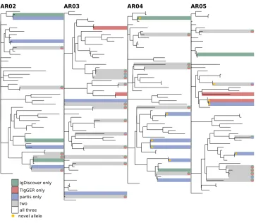
![FIGUREMK-type Myasthenia Gravis samples from [34] S3.Comparison of all three inference methods on the (explanation inFigure 8).](https://thumb-ap.123doks.com/thumbv2/123dok/2114496.1609207/33.612.126.488.104.369/figuremk-myasthenia-gravis-samples-comparison-inference-explanation-infigure.webp)
