Generating behavioral acts of predetermined apparent
complexity
A.V. Olifer
School of Science and Technology, Georgia Gwinnett College, 1000 University Center Lane, Lawrenceville, GA 30043, USA
Abstract
Behavior of natural and artificial agents consists of behavioral episodes or acts. This study introduces a quantitative measure of behavioral acts – their apparent complexity. The measure is based on the concept of the Kolmogorov complexity. It is an apparent measure because it is determined solely by the readings of the signals that directly encode percepts and actions during behavior. The article describes an algorithm of generating behavioral acts of predetermined apparent complexity. Such acts can be used to evaluate and develop learning abilities of artificial agents.
Keywords:
1. Introduction
Achievements of artificial intelligence often relate to specific tasks, for exam-ple winning the game of Go (AlphaGo, Google DeepMind) or interacting with people (robot Sophia, Hanson Robotics). The next step could be the agents able to learn tasks of any nature provided the behavior required for attaining the task is possible with the sensors and actuators the agents have. For example, Sophia’s descendants may not just talk but also play Go by moving stones on the board.
To develop such agents it might be beneficial to have achievable tasks of various complexity so that agents could gradually advance in learning. A related goal is to create measures and tests for evaluating and comparing agents [9, 8, 10, 13]. Known tasks often stimulate designing agents for task-specific behaviors (reviewed in [7]). The complexity of these tasks is defined in task-specific ways as well (finding goal from one direction, etc. [6]). Such measures of complexity cannot be applied to the tasks of different nature.
Complex tasks are associated with complex acts of behavior required to ac-complish the tasks’ goals. The present study focuses on the apparent complexity
Email address: [email protected](A.V. Olifer)
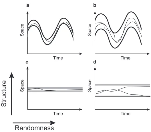
of behavioral acts. By apparent complexity we understand the complexity of readings of the agent’s sensors and actuators. Intuitively, the behavioral act is complex if the time series of the readings that are associated with the act 1) have few or no patterns, 2) are long, and 3) cannot vary or can vary only a little from one instance of the act to another, that is the behavior needs to be accurate. These three properties reflect the structure and randomness of a behavioral act (Fig.1). This general view (see, e.g., [15]) is put into work here using the Kolmogorov complexity.
The Kolmogorov complexity of an object, in this case a behavioral act, is es-sentially the length of its smallest possible description [11]. The concept has two issues related to the present subject. The first one is the incomputability of the Kolmogorov complexity. It means that in general the Kolmogorov complexity cannot be calculated exactly. However there are computable approximations of the Kolmogorov complexity that proved to be useful in various applied fields [4]. The second issue is that real-world individual behavioral acts have variability of sensory inputs and actions. To take this into account one needs to consider the Kolmogorov complexity not of one instance of the behavioral act but of the set of all possible instances.
Accordingly, two main assumptions are made here. First, that the readings of the sensors and actuators encoding rewards, percepts, and actions are fully known for every behavioral instance. Second, that the set of feasible behav-ioral instances of the act is either known or can be approximated. Explicit agent-environment interactions [7, 10] as well as the processes of learning and behavioral control are not considered in the present study.
The complexity of time series has been intensely studied using Information Theory methods [2, 12]. One approach is to accumulate statistics of a behavior and then use the Information Theory to quantify how predictive the behavior is [2, 12]. Simple behaviors are easily predicted and vise versa. The main difference between the proposed approach and Information Theory methods is in the focus of analysis. Information Theory methods strive to quantify the complexity of the process or the model generating a set of time series. The Kolmogorov complexity evaluates how hard is to compute or describe an individual series.
In this not we describe how to evaluate the complexity of behavioral acts and generate acts of predetermined complexity. The provided algorithm and examples show that acts of predetermined complexity can be generated using moderate computational resources.
2. Background
Time
Figure 1: Structure and randomness of behavior. Schematic representation of how two fun-damental characteristics of sets of objects, structure and randomness, distinguish behavioral acts. Behavior (a) has a relatively complex structure and allows only small random distor-tions. Behavior (b) has a relatively complex structure but allows larger distortions than in (a). Behavior (c) has a simple structure and allows only small distortions. Behavior (d) has a simple structure and allows large random distortions. ”Space” is an abstract space in which behaviors are defined; thick lines - borders of feasible behaviors, thin lines - instances of behaviors.
glands. In artificial agents, rewards, percepts, and actions are represented by the readings of the corresponding sensors and actuators.
Each of the three components of the act has its own complexity. For example, complex percepts may require simple actions, and so on. The complexity of each component is determined by the complexity of that component in a typical instance of the act and by the number of possible variations of that component in the feasible behavioral instances. For example, if the component in a typical instance is simple, and multiple variations in the feasilble instances are possible – the complexity of this component of the act is intuitively small (Fig.1d). On the contrary, if the component in a typical instance is complex, and only few variations of that component are possible – the complexity of this component of the act is intuitively large (Fig.1a).
description ofxand then halts. A rigorous definition, along with the proofs of the properties of the Kolmogorov complexity considered below, can be found in the encyclopedic treatise by Li and Vit´anyi [11].
The Kolmogorov complexity is not computable [11]. Analytical estimates of the Kolmogorov complexity often employ the fact that if the elements of a setS
are indexed then the index of an element has the length of at most⌈log|S|⌉bits. Here |S| is the cardinality of S, the logarithm as all the logarithms onwards is base two, and ⌈·⌉ is the ceiling function. In estimates of the Kolmogorov complexity, the error introduced by omitting the ceiling function is ignored.
To obtain a numerical estimate of the Kolmogorov complexity of a bitstring the file with the string is compressed. The length of the compressed file is taken as an estimate of the Kolmogorov complexity. This study uses gzip archiver for compressing. At the initial stage we also used bzip2 and got similar results in agreement with observations of others [4].
The following examples illustrate strengths and weaknesses of using gzip to approximate the Kolmogorov complexity.
Example 1: A 1024 byte–long random bitstring after compression by gzip became 1053 bytes long. The result of 1053 bytes was the same for several files with independent random bitstrings. The Kolmogorov complexity of a random bitstring cannot be less than the length of the string since there are no patterns to compress. The file length after compression increased compared to the original length since gzip needs extra bytes, in particular an eight-byte footer with a checksum.
Example 2: A 1024 byte–long file of zeros in every bit was compressed to 35 bytes. 35 bytes is longer than the two bytes needed to represent 213, the
number of bits in 1024 bytes, yet the level of compression is quite high because of the apparent simplicity of the bitstring of zeros.
Example 3: Letbi andbj,i < j, be two successive bits equal to one,bi= 1,
bj = 1, with the bits in between equal to zero, bk = 0, k = i+ 1,· · ·, j−1.
Transform the original string so that bi = 1, bj = 1, but bk = 1, k = i+
1,· · ·, j−1. In other words bits equal to one in the first string are considered as the endpoints of the intervals of the bits equal to one in the transformed string. For example, ’010010..’ transforms into ’011110..’ and so on. This transformation does not change the length of compressed files considerably. For example, a file of 1024 bytes with 1310 random bits equal to one was compressed to 769 bytes. The second file, with the transformed bitstring, was compressed to 735 bytes. The lengths of the files with bitstrings transformed in this way never differed for more than 5%.
3. Apparent complexity of behavioral acts
In what follows we define how to evaluate the complexity of actions. The other two components of behavioral acts, perceptions and rewards, are evaluated in the same way.
{0,1}nA, the set of all bitstrings of lengthn
A. Without loss of generality it is
further assumed thatA={0,1}nA. Time is discretized as well. At any moment
of time, the state of all the actuators is represented by a point inA.
Suppose a behavioral act lastsT time steps andM instances of it have been observed. LetAobs={a1, a2,· · · , aM}be the set of the corresponding actions.
Each instanceaj is a bitstring of the lengthn
A×(T+ 1). Next, letA denote
the set of all possible feasible actions associated with the act,Aobs⊆A; if the
act requires accurate movements then|A|, the cardinality ofA, should be small. Finally, letK(a) be the Kolmogorov complexity ofa∈A.
The following definition reflects the intuition that low accuracy of actions decreases the complexity of actions associated with the act and vice versa.
Definition 1. The complexity of actionsAassociated with an act is
C(A) =max(meana∈AK(a)−log|A|,0). (1)
This definition follows from a fundamental equality [11, p. 403],
K(S) +log|S|=K(x) +O(1),
showing that a minimal description of a typical representativexof a setSup to a constant that does not depend onxconsists of the minimal description ofS
and the minimal description ofxin S; the latter does not exceedlog|S|. Max-imization in (1) guarantees non-negativity ofC(A). According to (1), sampled instances allow only for an estimate ofC(A).
Definition 1 bears similarity with the definition of the complexity based on Predictive Information. Both contrast randomness and predictability [2]. We hypothesize both definitions are equivalent in an asymptotic sense.
The following example illustrates an application of (1).
Example 4: Consider two sets of 1024 byte-long bitstrings. In the bitstrings of the first set,S1, the first four bits in every byte are filled randomly with zeros and ones while the last four bits are always set to ones. An example would be ’01101111 11011111 ...’ . In the bitstrings of the second set, S2, the first byte is filled with ones and zeros exactly as in setS1. However all subsequent byte are not random. In each of them the first four bits are obtained from the first four bits of the previous byte by a cyclic permutation. As inS1, the last four bits are ones in every byte. For example, if the first byte was ’00111111’ then the second byte would be ’01101111’, the third one ’11001111’, and so on.
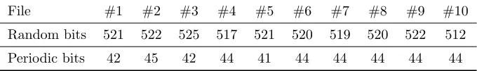
Suppose sets S1 and S2 correspond to the actions of the agent during two different behavioral acts. Which act requires more complex actions? Table 1 shows the lengths (in bytes) of ten randomly generated strings of S1 and
Table 1: The compressed length, in bytes, of two types of files. The files of the first type, ”Random bits”, had random values of the first four bits in every byte. The files of the second type, ”Periodic bits”, had repeated first four bits with the period of four bytes. The last four bits in every byte were equal to one in all the files. Before compression, every file had the length of 1024 bytes. The lengths after compression: mean = 519.9 bytes, std = 3.5 bytes for ”Random bits”; mean = 46.9 bytes, std = 1.6 bytes for ”Periodic bits”; n = 10.
File #1 #2 #3 #4 #5 #6 #7 #8 #9 #10
Random bits 521 522 525 517 521 520 519 520 522 512
Periodic bits 42 45 42 44 41 44 44 44 44 44
was equal to 4159 bits (4159 = 519.9×8). For S2, the mean complexity was equal to 347 bits (347 = 43.4×8). This shows that the elements ofS1 were on average more than ten times complex than the elements of S2. But what are the cardinalities of these sets? In the case of S1 there are 16 possible different combinations of 4 bits in each of 1024 bytes. It gives the total of 24·1024
possible instances. Thus |S1| = 24096, log|S1| = 4096 bits, and according to
(1), C(S1) = 4159−4096 = 63 bits. In contrast, |S2| is small. It has only 16 instances defined by the possible combinations of the first four bits. Hence
log|S2|= 4 bits, andC(S2) = 347−4 = 343 bits, which is about 5.5 times more than C(S1). Thus the second behavioral act, S2, is more complex compared to S1. The ”structural” component of S2 is relatively simple because of the periodicity. Its ”randomness” is low since only small variability in actions is allowed.
The complexity of rewards and percepts of behavioral acts can be evaluated in the same way as the complexity of actions. Together, they determine the complexity of the behavioral act.
Let R, P, and A be subsets of the reward space R, percept space P, and action spaceArespectively.
Definition 2. The complexity of a behavioral act(R, P, A)is the triple(C(R), C(P), C(A)), where C(R), C(P), and C(A) are the Kolmogorov complexities of the sets R,
P, andA defined according to (1).
4. Actions of predetermined complexity
This section describes how to generate components of behavioral acts with a predetermined complexity. Actions are considered for specificity. The other components are generated in the same way.
According to Definition 1, the complexity of actions is defined by two com-ponents: the complexity of a typical time series of actions and the cardinality of the set of all possible actions consistent with the act. The cardinality is assumed to be known. Then a sufficient complexity K of a typical time series follows from (1). First we show how to generate a time series with the complexity equal toK; it must be understood that in this and other cases the Kolmogorov complexity of an object can be determined only approximately. The value of the cardinality is then used to define possible distortions of the generated time series.
A bitstring of predetermined complexity can be obtained by assigning a certain number of randomly selected bits to one while keeping all the other bits equal to zero. LetLbe the number of bits equal to one in a bitstringsof length
n. There are Ln
of such strings. To describesit is suffice to describe the index of s in the set of nL
possible indexes. The description of the index takes no more thanlog nL
bits. The value ofLis determined from the requirement that the description length is the smallest among those exceedingK:
L= arg minL′{log
n
L′
≥K}. (2)
First of all, the inequality in (4) shows that to be complex, the string has to be long enough. Indeed, the inequality has no solutions for n such that
n n/2
≤ 2K. If L satisfies (4) then n−L also satisfies (4). This symmetry
reflects the fact that when all the zeros and ones in string s are flipped, the complexity ofsdoes not change.
In practice, one can findL from (4) using the bisection method. Binomial coefficients increase monotonically whenL′changes from 0 ton/2. The method
will require at mostlog(n) iterations.
Asymptotically, inequality (4) turns into an inequality with an entropy. Namely, suppose n is large and L ∼ λn and K ∼ κn for large n; here L is the solution to (4) . Then the approximation of the factorials in the binomial coefficient in (5) using Stirling’s formulan!∼√2πnnne−n yields
H(λ)≥κ, (3)
whereH(λ) =−λlog λ−(1−λ)log(1−λ)}. A minimalλthat satisfies (3) can be used an an (initial) approximation toL.
The same approach can be used for time series of strings. If there are no limitations on the number of bits equal to one at every time step, then allsican
one can be determined according to (4). formula leads to inequality (3) as well (just considern(T + 1) instead ofn). If the number of ones L at all of T+ 1 time step should be the same, then L is
On average, a time series consisting of T + 1 strings of length n with L bits equal to one in each of them is more complext compared to the string of length
n(T + 1) withL(T+ 1) bits equal to one since
In other words, on average the complexity of a string of length n(T + 1) bits can be achieved with a smaller number of bits equal to one if these bits are equaly spread betweenT+ 1 substrings of lengthn.
Interestingly, however, for large values ofnthe difference between the corre-sponding entropies vanishes. Indeed, assumingL∼λnandK∼κn(T+1) when
nis large and applying the Stirling formula to the multinomial the inequality (5) leads to the same inequality (3) for λ. In other words, asymptotically, λ, the average probability that a randomly selected bit is equal to one, could be the same.
The above formulas can be directly generalized for the case in which the number of bits equal to one in each si could be equal to Li, 0 ≤ Li ≤ n,
proximation of the multinomial coefficient in (5) using the Stirling’s formula yields:
H(λ)≥κ, (7)
whereH(λ) =PT
i=0H(λi) =PTi=0{−λilog λi−(1−λi)log(1−λi)}.
one can determine possible distortions of that series. Since this is going to be a ”staged” behavioral act it is assumed that|A| is known.
ALGORITHM
Require: C(A) – the target complexity of the set of actions A, |A| – the cardinality of A, nA – the number of bits at every time step, T – the number
of time steps,R - the set of possible values of the number of ones. 1. CalculateK=C(A) +log|A|; cf. (1).
2. Check ifT andnAare sufficiently large. If the inequality (7) holds
then CONTINUE, else STOP.
3. Determine the number of bits to be assigned to one, using formulas (6), (5), or (4).
4. Generate a sequence of strings of complexityK by assigning to one the number of bits, obtained in 3., in random positions. Set other bits to zeros.
Example 5: In this example, the goal was to use the algorithm to generate time series that could be considered as typical action instances for the action with the complexityC(A) = 2048 bits and the number of bits at every time step
nA = 8. The number of bits equal to one, n1A, was determined for the whole
time series. Bitstrings, representing typical instances of the actions, varied from trial to trial. The lengths of the corresponding compressed files varied as well. However, the variances of the lengths were small.
For the first action, the input wasC(A) = 2048 bits, nA= 8 bits,T = 255,
|A|= 0. Step 1 resulted in K = 2048. In Step 2, the value ofT was found to satisfynA(T + 1) =K. In Step 3, n1A was found according to (4) to be equal
to n1
A = 0.5nA = 1024 bits. In step 4, bits were set to one with probability
0.5, which resulted in 1026 bits equal to one (Fig.2a). The corresponding file was compressed to 2280 bits. By construction (|A|= 0) , distortions were not allowed for this particular action.
For the second action, the input was C(A) = 2048 bits, |A| = 0, nA = 8
bits, T = 1023. Step 1 resulted in K = 2048. In Step 2, the value of T was found to satisfynA(T+ 1)> K. In Step 3,n1A= 344 bits was found according
to (4). In step 4, bits were set to one with the probability 0.042 = 344/8192, which resulted in 349 bits equal to one (Fig.2b). The corresponding file was compressed to 3328 bits. By construction, distortions were not allowed for this particular action.
For the third action, the input was C(A) = 2048 bits,|A|= 22048,n
A = 8
bits,T = 1023. Note that in this case distortions were allowed. Step 1 resulted inK= 4096. In Step 2, the value ofT was found to satisfynA(T+ 1)> K. In
Step 3, n1
A = 912 bits was found according to (4). In step 4, bits were set to
one with the probability 0.111 = 912/8192, which resulted in 886 bits equal to one (Fig.2c). The corresponding file was compressed to 5312 bits.
case,A =B(N, ρ) is the ball of radiusρin the space {0,1}N, N =n(T+ 1),
centered at the point represented by a typical action instance. To determine the radius of the ball one can use the Hamming distance. The Hamming distance between binary strings equals to the number of bits, in which the values of the two strings differ. In this case, if the radius ρ =pN, 0 < p ≤0.5, then |V| ≤2H(p)N, where H(p) is the binary Shannon’s entropyH(p) = −p log p−
(1−p)log(1−p) [5, p. 52]. It is easy to find thatH(p) = 0.25 whenp≈0.04. It implies that the ball has no more than|A|= 22048 = 20.25∗8192 elements if the
radius does not exceed 327 =⌊0.04∗8∗1024⌋; here ⌊·⌋ is the floor operation. Hence, other actions corresponding to the case considered, can be at distance of at most 327 bits from the sequence shown in (Fig.2c). These actions can be obtained by flipping at most 327 randomly chosen bits in the sequence from (Fig.2c). Fig.2c relates to Fig.2b as Fig.1b relates to Fig.1a.
c
0 bits 2048 8192
b
0 bits 2048 8192
a
0 bits 2048
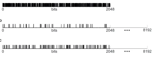
Figure 2: Actions of predetermined complexity. The target complexity of actions was 2048 bits. (a) An action, represented by a completely random bitstring of length 2048 bits. The probability of bits equal to one equals 0.5. Distortions are not allowed. (b) An action, represented by a bitstring of length 8192 bits. The probability of ones equals 0.042. The string has the complexity close to 2048 bits. Distortions are not allowed. (c) An action, represented by a string of length 8192 bits. The probability of ones equals 0.111. The complexity of the string is about 4096 bits. This action allows for distortions. Other feasible actions can differ from the represented action in no more than 327 bits. Because of the allowed distortions the action has complexity close to 2048 bits as in (a) and (b).
5. Discussion
An algorithm of generating possible descriptions of behavioral acts of predeter-mined complexity is reported. Using the algorithm, one can generate abstract sequences of rewards, percepts and actions that would represent successful be-havior. Machines could be tested in learning and performing the tasks which are defined by all three components. The work of the algorithm is demonstrated on several examples.
Rewards, percepts and actuators of one and the same behavioral act have their own complexities, though the number of time steps for those time series is obviously the same. The components may have different complexity of typ-ical instances and allowed variability (Fig.2). The effects of these factors on behavioral complexity can be taken into account in studies of animals and com-parison and testing of artificial agents. In animals, it would be interesting to evaluate complexities of behavioral acts and their relative frequencies to better undestand what the brain does for survival of those animals.
Comparison of apparent behaviors does not require exactly the same number and characteristics of sensors and actuators in the compared agents. For the agents with smaller dimensions of sensory and actuators spaces extra dimensions can be formally added. Adding zero readings in those dimensions adds only a little to the Kolmogorov complexity.
It would be also interesting to evaluate known behavioral tasks for artificial agents, from grabbing objects to playing computer games, to playing Go. For artificial agents all the data, required to evaluate complexity, is available. For example, in the case of neural networks ”playing” computer games [1] the time series of rewards are the game points, percepts are the signals from the monitor, and actions are the codes of the joystick. In this example, one of the questions to explore would be about the relation of the network performance to the com-plexity of the behavior. Intuition suggests that at least some behavioral acts in agents and animals can be compared according to the lexicographic order of the triples (C(R), C(P), C(A)), where C(R), C(P), and C(A) are the complexity of rewards, percepts, and actions respectively. Is it really the case for computer games? Some games can be associated with sets of behavioral acts. For exam-ple, in chess a behavioral act is a won game. In such cases the overall complexity of the game can be defined as an average complexity of the corresponding acts. A fundamental limitation of the proposed approach is the incomputability of the Kolmogorov complexity [11] which is akin to undersampling in the in-formation theoretic approach [12]. The lengths of compressed files overestimate the complexity. It has to be taken into account.
In the analysis of animal behavior, the approach is limited by the ability of obtaining the readings of sensors and actuators. For simple behaviors, such as reaching for an object by a monkey, only subsets of sensors and actuators can be considered. However, the most critical readings can already be evalu-ated relatively well [14]. In the future, more detailed measurements should be possible.
instances can have arbitrary geometry. In particular, they can form unions of two or more disjoint nonempty subsets. To account for this, one can can consider the ratio of the boundary area to the volume of the sets.
Another direction is to generate a time series of predetermined complexity using patterns. The method, described in this study, is to set some bits to one randomly. However, even for artificial agents not all combinations of bits are feasible. The approach should be therefore adjusted to using only feasible pat-terns. Development in this direction is likely related to the studies of grammar complexity (see, e.g. [3]).
Acknowledgements
The author thanks Dr. Peter Erdi and Dr. Lance Fortnow for valuable discussions.
References
[1] Bellemare, M.G., Naddaf, Y., Veness, J., Bowling, M.. The arcade learning environment: An evaluation platform for general agents. J Artif Intell Res(JAIR) 2013;47:253–279.
[2] Bialek, W., Nemenman, I., Tishby, N.. Predictability, complexity, and learning. Neural computation 2001;13(11):2409–2463.
[3] Charikar, M., Lehman, E., Liu, D., Panigrahy, R., Prabhakaran, M., Rasala, A., Sahai, A., Shelat, A.. Approximating the smallest grammar: Kolmogorov complexity in natural models. In: Proceedings of the Thiry-fourth Annual ACM Symposium on Theory of Computing. New York, NY, USA: ACM; STOC ’02; 2002. p. 792–801.
[4] Cilibrasi, R., Vit´anyi, P.M.. Clustering by compression. IEEE Transactions on Information theory 2005;51(4):1523–1545.
[5] Cover, T., Thomas, J.. Elements of Information Theory. John Wiley & Sons, Inc., 1991.
[6] Franz, M.O., Mallot, H.A.. Biomimetic robot navigation. Robotics and au-tonomous Systems 2000;30(1):133–153.
[7] Hern´andez-Orallo, J.. On environment difficulty and discriminating power. Au-tonomous Agents and Multi-Agent Systems 2015;29(3):402–454.
[8] Hern´endez-Orallo, J.. Beyond the turing test. Journal of Logic, Language and Information 2000;9(4):447–466.
[10] Legg, S., Veness, J.. An approximation of the universal intelligence measure. In: Algorithmic Probability and Friends. Bayesian Prediction and Artificial In-telligence. Springer; 2013. p. 236–249.
[11] Li, M., Vit´anyi, P.M.. An Introduction to Kolmogorov Complexity and Its Applications. 3rd ed. Springer, 2008.
[12] Palmer, S.E., Marre, O., Berry, M.J., Bialek, W.. Predictive informa-tion in a sensory populainforma-tion. Proceedings of the Nainforma-tional Academy of Sciences 2015;112(22):6908–6913.
[13] Schmidhuber, J.. The speed prior: a new simplicity measure yielding near-optimal computable predictions. In: International Conference on Computational Learning Theory. Springer; 2002. p. 216–228.
[14] Scott, S.H.. Optimal feedback control and the neural basis of volitional motor control. Nature Reviews Neuroscience 2004;5(7):532–546.