Evolutionary dynamics and competition stabilize
three-species predator-prey communities
Sheng Chena, Ulrich Dobramyslb, Uwe C. T¨aubera
a
Department of Physics (MC 0435) and Center for Soft Matter and Biological Physics, Robeson Hall, 850 West Campus Drive, Virginia Tech, Blacksburg, Virginia 24061, USA
b
Wellcome Trust / Cancer Research UK Gurdon Institute, University of Cambridge, Cambridge CB2 1QN, United Kingdom
Abstract
We perform individual-based Monte Carlo simulations in a community
consist-ing of two predator species competconsist-ing for a sconsist-ingle prey species, with the purpose
of studying biodiversity stabilization in this simple model system. Predators
are characterized with predation efficiency and death rates, to which Darwinian
evolutionary adaptation is introduced. Competition for limited prey abundance
drives the populations’ optimization with respect to predation efficiency and
death rates. We study the influence of various ecological elements on the final
state, finding that both indirect competition and evolutionary adaptation are
insufficient to yield a stable ecosystem. However, stable three-species
coexis-tence is observed when direct interaction between the two predator species is
implemented.
Keywords: Darwinian evolution, interspecific competition, Lotka-Volterra
model, multi-species coexistence, character displacement
1. Introduction
Ever since Darwin first introduced his theory that interspecific competition
positively contributes to ecological character displacement and adaptive
diver-∗Corresponding author: Ulrich Dobramysl, [email protected], Wellcome
Trust / Cancer Research UK Gurdon Institute, University of Cambridge, Cambridge CB2 1QN, United Kingdom
Email addresses: [email protected](Sheng Chen),[email protected](Ulrich Dobramysl),[email protected](Uwe C. T¨auber)
gence [1], debates abounded about its importance in biodiversity. Character
displacement is considered to occur when a phenotypical feature of the animal
[2], which could be morphological, ecological, behavioral, or physiological, beak
size for example, is shifted in a statistically significant manner due to the
intro-duction of a competitor [3, 4]. One example of ecological character displacement
is that the body size of an island lizard species becomes reduced on average upon
the arrival of a second, competing lizard kind [5]. Early observational and
ex-perimental studies of wild animals provided support for Darwinian evolutionary
theory [6, 2]. One famous observation related to finches, whose beak size would
change in generations because of competition [6]. However, recent studies
us-ing modern genetic analysis techniques do not find genetic changes to the same
extent as the phenotypic break change, thereby casting doubt on Darwin’s
ob-servational studies [7, 8]. Another concern with experiments on birds or other
animal species is that they may live for decades, rendering this sort of study
too time-consuming. Evolutionary theory is based on the assumption that
in-terspecific competition occurs mostly between closely related species because
they share similar food resources, thus characters exploiting new resources are
preferred. Ecologists perform experiments with wild animals by introducing a
second competing species and recording their observable characters including
the body size, beak length, and others [8, 5]. Unfortunately, direct control over
natural ecosystems is usually quite limited; for example, ecological character
dis-placement with wild animals cannot be shut down at will in natural habitats.
However, this is easily doable in carefully designed computer simulations.
Game theory has a long history in the study of biological problems [9].
Among all the mathematical models of studying biodiversity in ecology, the
Lotka–Volterra (LV) [10, 11] predator-prey model may rank as possibly the
simplest one. Only one predator and one prey species are assumed to exist
in the system. Individuals from each species are regarded as simple particles
with their reaction rates set uniformly and spatially homogeneous. They
dis-play three kinds of behaviors which are influenced by pre-determined reaction
and predators may remove a prey particle and simultaneously reproduce. This
simple LV model kinetics may straightforwardly be implemented on a regular
lattice (usually square in two or cubic in three dimensions) to simulate situations
in nature, where stochasticity as well as spatio-temporal correlations play an
im-portant role [12]–[27]. It is observed in such spatial stochastic LV model systems
that predator and prey species may coexist in a quasi-stable steady state where
both populations reach non-zero densities that remain constant in time; here,
the population density is defined as the particle number of one species divided
by the total number of lattice sites. Considering that the original LV model
contains only two species, we here aim to modify it to study a multi-species
system. We note that there are other, distinct well-studied three-species
mod-els, including the rock-paper-scissors model [28, 30], which is designed to study
cyclic competitions, and a food-chain-like three-species model [29], as well as
more general networks of competing species [30], all of which contain species
that operate both as a predator and a prey. In this paper we mainly focus
on predator-prey competitions, where any given species plays only one of those
ecological roles.
Compared with the original LV model, we introduce one more predator into
the system so that there are two predator species competing for the same prey.
We find that even in a spatially extended and stochastic setting, the ‘weaker’ of
the two predator species will die out fast if all reaction rates are fixed.
After-wards the remaining two species form a standard LV system and approach stable
steady-state densities. Next we further modify the model by introducing
evo-lutionary adaptation [31]. We also add a positive lower bound to the predator
death rates in order to avoid ‘immortal’ particles. Finally, we incorporate
addi-tional direct competition between predator individuals. Stable multiple-species
coexistence states are then observed in certain parameter regions,
demonstrat-ing that adaptive ‘evolution’ in combination with direct competition between
the predator species facilitate ecosystem stability. Our work thus yields insight
into the interplay between evolutionary processes and inter-species competition
2. Stochastic lattice Lotka–Volterra Model with fixed reaction rates
2.1. Model description
We spatially extend the LV model by implementing it on a two-dimensional
square lattice with linear system sizeL= 512. It is assumed that there are three
species in the system: two predator speciesA, B, and a single prey speciesC.
Our model ignores the detailed features and characters of real organisms, and
instead uses simple ‘particles’ to represent the individuals of each species. These
particles are all located on lattice sites in a two-dimensional space with
peri-odic boundary conditions (i.e., on a torus) to minimize boundary effects. Site
exclusion is imposed to simulate the natural situation that the local population
carrying capacity is finite: Each lattice site can hold at most one particle, i.e., is
either occupied by one ‘predator’AorB, occupied by one ‘prey’C, or remains
empty. This simple model partly captures the population dynamics of a real
eco-logical system because the particles can predate, reproduce, and spontaneously
die out; these processes represent the three main reactions directly affecting
population number changes. There is no specific hopping process during the
simulation so that a particle will never spontaneously migrate to other sites.
However, effective diffusion is brought in by locating the offspring particles on
the neighbor sites of the parent particles in the reproduction process [25, 27].
The stochastic reactions between neighboring particles are described as follows:
A µA
−−→ ∅, B µB −−→ ∅,
A+C λA
−−→A+A , B+C λB
−−→B+B ,
C−→σ C+C .
(1)
The ‘predator’ A (or B) may spontaneously die with decay rateµA(µB) >0.
The predators may consume a neighboring prey particleC, and simultaneously
reproduce with ‘predation’ rateλA/B, which is to replaceCwith a new predator
particle in the simulation. In nature, predation and predator offspring
qualitative differences in a stochastic spatially extended system in dimensions
d <4 [24]. When a prey particle has an empty neighboring site, it can
gen-erate a new offspring prey individual there with birth rateσ > 0. Note that
a separate prey death process C → 0 can be trivially described by lowering
the prey reproduction rate and is therefore not included. We assume asexual
reproduction for all three species, i.e., only one parent particle is involved in
the reproduction process. Each species consists of homogeneous particles with
identical reaction rates. Predator speciesAand B may be considered as close
relatives since they display similar behavior (decay, predation and reproduction,
effective diffusion) and most importantly share the same mobile food sourceC.
For now, we do not include evolution in the reproduction processes, therefore
all offspring particles are exact clones of their parents. We are now going to
show that these two related predator species can never coexist.
2.2. Mean-field rate equations
The mean-field approximation ignores spatial and temporal correlations and
fluctuations, and instead assumes the system to be spatially well-mixed. We
definea(t) and b(t) as the predators’ population densities and c(t) as the prey
density. Each predator population decreases exponentially with death rateµ,
but increases with the predation rateλand prey densityc(t). The prey
popula-tionc(t) increases exponentially with its reproduction rateσ, but decreases as
a function of the predator population densities. The mean-field rate equations
consequently read
da(t)
dt =−µAa(t) +λAa(t)c(t), db(t)
dt =−µBb(t) +λBb(t)c(t), dc(t)
dt =σc(t)
1−a(t) +b(t) +c(t)
K
−λAa(t)c(t)−λBb(t)c(t).
(2)
K >0 represents the finite prey carrying capacity. In order to obtain stationary
densities, the left-side derivative terms are set to zero. The ensuing (trivial)
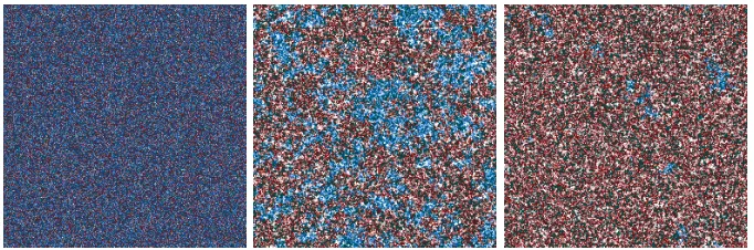
Figure 1: Snapshots of the spatial particle distribution for a single Monte Carlo simulation
run of a stochastic predator-predator-prey Lotka–Volterra model on a 512×512 square lattice
with periodic boundary conditions at (from left to right)t= 0 Monte Carlo Steps (MCS),
t= 10 000 MCS, andt= 50 000 MCS, with predation ratesλA = 0.5,λB = 0.5, predator
death ratesµA= 0.126,µB= 0.125, and prey reproduction rateσ= 1.0. Only at most one
particle per lattice site is allowed. Predator particlesAare indicated in blue, predatorsBin red, and preyCin dark green, while empty sites are shown in white.
µA< λAK: a=σλ(A(λAλKAK−+µA)σ), b= 0,c=µA/λA; (4) forµB < λBK: a= 0,b=
σ(λBK−µB)
λB(λBK+σ), c=µB/λB. WhenµA/λA 6=µB/λB, there exists no three-species
coexistence state. Yet in the special situationµA/λA=µB/λB, another line of
fixed points emerges: (σ
K +λA)a+ ( σ
K +λB)b+ σ
Kc=σ,c=µA/λA=µB/λB.
2.3. Lattice Monte Carlo simulation results
In the stochastic lattice simulations, population densities are defined as the
particle numbers for each species divided by the total number of lattice sites
(512×512). We prepare the system so that the starting population densities
of all three species are the same, here set to 0.3 (particles/lattice site), and the
particles are initially randomly distributed on the lattice. The system begins to
leave this initial state as soon as the reactions start and the ultimate
station-ary state is only determined by the reaction rates, independent of the system’s
initialization. We can test the simulation program by setting the parameters
as λA = λB = 0.5 and µA = µB = 0.125. Since species A and B are now
exactly the same, they coexist with an equal population density in the final
stable state, as indeed observed in the simulations. We increase the value of
shows the spatial distribution of the particles at 0, 10 000, and 50 000 Monte
Carlo Steps (MCS, from left to right), indicating sites occupied byAparticles
in blue, B in red, C in green, and empty sites in white. As a consequence of
the reaction scheme (1), specifically the clonal offspring production, surviving
particles in effect remain close to other individuals of the same species and thus
form clusters. After initiating the simulation runs, one typically observes these
clusters to emerge quite quickly; as shown in Fig. 1, due to the tiny difference
between the death ratesµA−µB>0, the ‘weaker’ predator speciesAgradually
decreases its population number and ultimately goes extinct. Similar behavior
is commonly observed also with other sets of parameters: For populations with
equal predation rates, only the predator species endowed with a lower
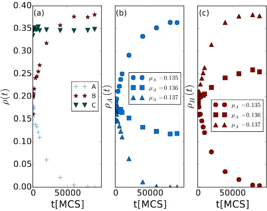
sponta-neous death rate will survive. Fig. 2(a) records the temporal evolution of the
three species’ population densities. After about 60 000 MCS, predator species
Ahas reached extinction, while the other two populations eventually approach
non-zero constant densities. With larger values of µA such as 0.127 or 0.13,
speciesAdies out within a shorter time interval; the extinction time increases
with diminishing death rate difference|µA−µB|.
In Figs. 2(b) and (c), we setλA= 0.55,λB = 0.5,µB = 0.125, and various
values of µA >0.13. The larger rate λA gives species A an advantage overB
in the predation process, while the bigger rate µA enhances the likelihood of
death for A as compared to B. Upon increasing µA from 0.135 to 0.137, we
observe a phase transition from speciesB dying out toA going extinct in this
situation with competing predation and survival advantages. When µA thus
exceeds a certain critical value (in this example near 0.136), the disadvantages
of high death rates cannot balance the gains due to a more favorable predation
efficiency; hence predator species A goes extinct. In general, whenever the
reaction rates for predator species A and B are not exactly the same, either
Aor B will ultimately die out, while the other species remains in the system,
coexisting with the preyC. This corresponds to actual biological systems where
two kinds of animals share terrain and compete for the same food. Since there
0 50000
Figure 2: The two predator species cannot coexist in Monte Carlo simulations of the
two-predator-one-prey model with fixed reaction rates. (a) Time evolution of the population
densities with fixed reaction rates: predation ratesλA= 0.5,λB = 0.5, predator death rates
µA= 0.126,µB= 0.125, and prey reproduction rateσ= 1.0; (b,c) temporal evolution of the
population densitiesρA(t) and ρB(t) with fixedλA = 0.55,λB = 0.5,µB = 0.125, andµA
varying from 0.135, 0.136, to 0.137. The curves in (b) and (c) sharing the same markers are from the same (single) simulation runs.
population will gradually decrease. This trend cannot be turned around unless
the organisms improve their capabilities or acquire new skills to gain access
to other food sources; either change tends to be accompanied by character
displacements [32, 33, 34, 35].
In order to quantitatively investigate the characteristic time for the weaker
predator species to vanish, we now analyze the relation between the relaxation
time tc of the weaker predator species (A here) and the difference of death
rates |µA−µB| under the condition that λA = λB. Fig. 2(a) indicates that
prey density (green triangles) reaches its stationary value much faster than the
0 40000 80000
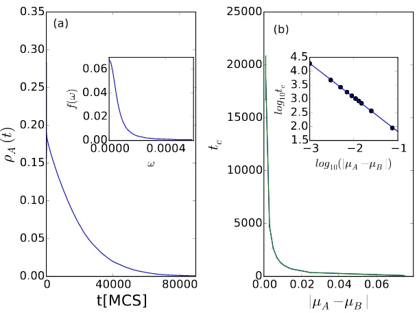
Figure 3: Characteristic decay time of the weaker predator species measured in Monte Carlo
simulations of the two-predator-one-prey model with fixed reaction rates. (a) Main panel:
temporal evolution of the predator population densityρA(t) with predation rates λA= 0.5,
λB= 0.5, predator death ratesµA= 0.126,µB= 0.125, and prey reproduction rateσ= 1.0.
Inset: Fourier transform amplitudef(ω) of the predator density time seriesρA(t). (b) Main
panel: characteristic decay timetcas obtained from the peak width off(ω), versus the death
rate difference|µA−µB|, with all other reaction rates fixed as in (a). Inset: the black dots
show the data points log10tcversus log10(|µA−µB|), while the blue straight line with slope −1.23±0.01 is inferred from linear regression.
to a two-species model, wherein the relaxation time of the prey speciesCis finite.
However, the relaxation time of either predator species would diverge because it
takes longer for the stronger species to remove the weaker one when they become
very similar in their death probabilities. Upon rewriting eqs. (2) forλA =λB
by replacing the prey density c(t) with its stationary value µB/λB, we obtain
a linearized equation for the weaker predator density: dadt(t) =−|µA−µB|a(t),
describing exponential relaxation with decay timetc= 1/|µA−µB|.
We further explore the relation between the decay rate of the weak species
Fig. 3(a) shows an example of the weaker predatorApopulation density decay
for fixed reaction rates λA = 0.5, λB = 0.5, µA = 0.126, µB = 0.125, and
σ = 1.0, and in the inset also the corresponding Fourier amplitude f(ω) =
|R e−iωtρ
A(t)dt| that is calculated by means of the fast Fourier transform
al-gorithm. Assuming an exponential decay of the population density according
to ρA(t)∼ e−t/tc, we identify the peak half-width at half maximum with the
inverse relaxation time 1/tc. For other values of µA > 0.125, the measured
relaxation timestc for the predator speciesA are plotted in Fig. 3(b). We also
ran simulations for various parameter valuesµA<0.125, for which the predator
populationB would decrease toward extinction instead ofA, and measured the
corresponding relaxation time forρB(t), plotted in Fig. 3(b) as well. The two
curves overlap in the main panel of Fig. 3(b), confirming that tc is indeed a
function of|µA−µB| only. The inset of Fig. 3(b) demonstrates a power law
relationship tc ∼ |µA−µB|−zν between the relaxation time and the reaction
rate difference, with exponentzν≈ −1.23±0.01 as inferred from the slope in
the double-logarithmic graph via simple linear regression. This value is to be
compared with the corresponding exponentzν≈1.295±0.006 for the directed
percolation (DP) universality class [36]. Directed percolation [38] represents a
class of models that share identical values of their critical exponents at their
phase transition points, and is expected to generically govern the critical
prop-erties at non-equilibrium phase transitions that separate active from inactive,
absorbing states [39, 40]. Our result indicates that the critical properties of the
two-predator-one-prey model with fixed reaction rates at the extinction
thresh-old of one predator species appear to also be described by the DP universality
class.
As already shown in Fig. 1, individuals from each species form clusters in the
process of the stochastically occurring reactions (2). The correlation lengthsξ,
obtained from equal-time correlation functions C(x), characterize the average
sizes of these clusters. The definition of the correlation functions between the
different species α, β = A, B, C is Cαβ(x) = hnα(x)nβ(0)i − hnα(x)ihnβ(0)i,
0 2 4 6 8 10 12 14
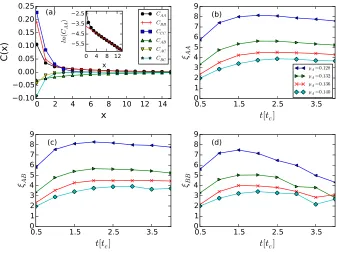
Figure 4: Time evolution for correlation lengths during Monte Carlo simulations of the
two-predator-one-prey model with fixed reaction rates. (a) Main panel: correlation functions
C(x) after the system has evolved for one half of the relaxation time 0.5tc≈2386 MCS, with
reaction ratesλA = 0.5,λB = 0.5,µA = 0.128,µB = 0.125, andσ= 1.0. Inset: ln(CAA)
with a simple linear regression of the data points withx∈[4,14] (red straight line) that yields the characteristic correlation decay lengthξAA≈5.8. (b,c,d) Measured correlation lengths
ξAA,ξAB, andξBB as function of the system evolution time t relative totc, with reaction
rates as in (a) except (top to bottom)µA = 0.128 (blue left triangles), 0.132 (green right
x. First choosing a lattice site, and then a second site at distance xaway, we
note that the productnα(x)nβ(0) = 1 only if a particle of speciesβ is located
on the first site, and a particle of speciesα on the second site; otherwise the
product equals 0. We then average over all sites to obtainhnα(x)nβ(0)i. hnα(x)i
represents the average population density of speciesα.
In our Monte Carlo simulations we find that although the system has not
yet reached stationarity at 0.5tc, its correlation functions do not vary
apprecia-bly during the subsequent time evolution. This is demonstrated in Figs.
4(b-d) which show the measured correlation lengths from 0.5tc to 3.75tc, during
which time interval the system approaches its quasi-stationary state. The main
panel in Fig. 4(a) shows the measured correlation functions after the system
has evolved for 0.5tc ≈ 2386 MCS, with predator A death rate µA = 0.128.
Individuals from the same species are evidently spatially correlated, as
indi-cated by the positive values of Cαα. Particles from different species, on the
other hand, display anti-correlations. The inset demonstrates exponential decay:
CAA(x)∼e−|x|/ξAA, whereξAAis obtained from linear regression ofln(CAA(x)).
In the same manner, we calculate the correlation lengthξAA,ξBB, andξAB for
every 0.5tc the system evolves, for different species Adeath ratesµA = 0.128,
0.132, 0.136, and 0.140, respectively. Fig. 4(b) shows that predator A clusters
increase in size by about two lattice constants within 1.5tc after the reactions
begin, and then stay almost constant. In the meantime, the total population
number of species A decreases exponentially as displayed in Fig. 3, which
in-dicates that the number of predator A clusters decreases quite fast. Fig. 4(c)
does not show prominent changes for the values ofξAB(t) as the reaction time
t increases, demonstrating that speciesA and B maintain a roughly constant
distance throughout the simulation. In contrast, Fig. 4(d) depicts a significant
temporal evolution of ξBB(t): the values of ξBB are initially close to those of
ξAA, because of the coevolution of both predator speciesAandB; after several
decay timestc, however, there are few predatorA particles left in the system.
The four curves forξBBwould asymptotically converge after speciesAhas gone
To summarize this section, the two indirectly competing predator species
cannot coexist in the lattice three-species model with fixed reaction rates. The
characteristic time for the weaker predator species to go extinct diverges as
its reaction rates approach those of the stronger species. We do not observe
large fluctuations of the correlation lengths during the system’s time evolution,
indicating that spatial structures remain quite stable throughout the Monte
Carlo simulation.
3. Introducing character displacement
3.1. Model description
The Lotka–Volterra model simply treats the individuals in each population
as particles endowed with uniform birth, death, and predation rates. This does
not reflect a natural environment where organisms from the same species may
still vary in predation efficiency and death or reproduction rates because of their
size, strength, age, affliction with disease, etc. In order to describe individually
varying efficacies, we introduce a new characterη∈[0,1], which plays the role of
an effective trait that encapsulates the effects of phenotypic changes and
behav-ior on the predation / evasion capabilities, assigned to each individual particle
[31]. When a predatorAi(orBj) and a preyCkoccupy neighboring lattice sites,
we set the probability (ηAi+ηCk)/2 [or (ηBj+ηCk)/2] forCkto be replaced by
an offspring predatorAz(orBz). The indicesi,j,k, andzhere indicate specific
particles from the predator populationsAorB, the prey populationC, and the
newly created predator offspring in either theAor B population, respectively.
In order to confine all reaction probabilities in the range [0,1], the efficiencyηAz
(orηBz) of this new particle is generated from a truncated Gaussian distribution
that is centered at its parent particle efficiency ηAi (or ηBj) and restricted to
the interval [0,1], with a certain prescribed distribution width (standard
devi-ation) ωηA (or ωηB). When a parent prey individual Ci gives birth to a new
offspring particleCz, the efficiencyηCz is generated through a similar scheme
parent’s efficacy but with some random mutational adaptation or
differentia-tion. The distribution width ω models the potential range of the evolutionary
trait change: for larger ω, an offspring’s efficiency is more likely to differ from
its parent particle. Note that the width parametersω here are unique for
par-ticles from the same species, but may certainly vary between different species.
In previous work, we studied a two-species system (one predator and one prey)
with such demographic variability [31, 37]. In that case, the system arrived at a
final steady state with stable stationary positive species abundances. On a much
faster time scale than the species density relaxation, their respective efficiency
η distributions optimized in this evolutionary dynamics, namely: the
preda-tors’ efficacies rather quickly settled at a distribution centered at values near 1,
while the prey efficiencies tended to small values close to 0. This represents a
coevolution process wherein the predator population on average gains skill in
predation, while simultaneously the prey become more efficient in evasion so as
to avoid being killed.
3.2. Quasi-species mean-field equations and numerical solution
We aim to construct a mean-field description in terms of quasi-subspecies
that are characterized by their predation efficaciesη. To this end, we discretize
the continuous interval of possible efficiencies 0≤η≤1 intoNbins, with the bin
midpoint valuesηi= (i+1/2)/N,i= 0, . . . , N−1. We then consider a predator
(or prey) particle with an efficacy value in the rangeηi−1/2≤η≤ηi+ 1/2 to
belong to the predator (or prey) subspeciesi. The probability that an individual
of speciesA with predation efficiencyη1 produces offspring with efficiency η2
is assigned by means of a reproduction probability function f(η1, η2). In the
binned version, we may use the discretized form fij =f(ηi, ηj). Similarly, we
have a reproduction probability functiongij for predator species B andhij for
the preyC. Finally, we assign the arithmetic meanλik= (ηi+ηk)/2 to set the
effective predation interaction rate of predatoriwith preyk[31, 37].
rate equations for the temporal evolution of the subspecies populations:
Steady-state solutions are determined by setting the time derivatives to zero,
∂ai(t)/∂t = ∂bi(t)/∂t = ∂ci(t)/∂t = 0. Therefore, the steady-state particle
counts can always be found by numerically solving the coupled implicit equations
µai=
In the special case of a uniform inheritance distribution for all three species,
We could not obtain the full time-dependent solutions to the mean-field
equa-tions in closed form. We therefore employed an explicit fourth-order Runge–
Kutta scheme to numerically solve eqs. (3), using a time step of ∆t= 0.1, the
initial conditionai(t= 0) = bi(t= 0) = ci(t = 0) = 1/(3N) fori = 1, ..., N, a
number of subspeciesN = 100, and the carrying capacityK = 1. An example
for the resulting time evolution of the predatorB density is shown in Fig. 5(b);
its caption provides the remaining parameter values.
3.3. Lattice simulation
We now proceed to Monte Carlo simulations for this system on a
two-dimensional square lattice, and first study the case where trait evolution is
solely introduced to the predation efficienciesη. In these simulation, the values
of µ and σ are held fixed, as is the nonzero distribution width ω, so that an
offspring’s efficiency usually differs from its parent particle. In accord with the
numerical solutions for the mean-field equations (3), we find that the
three-species system (predators A and B, prey C) is generically unstable and will
evolve into a final two-species steady state, where one of the predator species
goes extinct, depending only on the value ofω(given that µandσare fixed).
At the beginning of the simulation runs, the initial population densities,
which are the particle numbers of each species divided by the lattice site number,
are assigned the same value 0.3 for all the three species. The particles are
randomly distributed on the lattice sites. We have checked that the initial
conditions do not influence the final state by varying the initial population
densities and efficiencies. We fix the predator death rate toµ= 0.125 for both
speciesAandB, and set the prey reproduction rate asσ= 1.0. The predation
efficacies for all particles are initialized atη= 0.5. We have varied the values of
the distribution widthω and observed the final (quasi-)steady states. For the
purpose of simplification, we fixωηA=ωσC= 0.1, and compare the final states
when various values ofωηBare assigned.
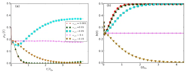
Fig. 5(a) shows the population density ρB(t) of predator species B with
0 1 2 3 4
Figure 5: (a) Stochastic lattice simulation of the two-predator-one-prey model with
‘Dar-winian’ evolution introduced only for the predation efficiencyη: predator population density
ρB(t) for various values of the predation efficiency distribution widthωηB= 0.001 (red dots),
0.01 (green triangles up), 0.05 (blue squares), 0.1 (pink crosses), and 0.15 (orange triangles down), with all other reaction rates held fixed atµ= 0.125,σ= 1.0, andωηA=ωηC = 0.1;
Monte Carlo time t rescaled with the relaxation time t0s = 1900 MCS of the curve for
ωηB = 0.05. (b) Numerical solution of the mean-field eqs. (3) withb(t) = N1 Pibi(t)
de-noting the average subspecies density. The parameters are set at the same values as for the
lattice simulations; timetis again normalized with the relaxation time t0 = 204.32 of the
curve forωηB = 0.05 curve to allow direct comparison with the simulation data. Note that
the limited carrying capacity in both lattice simulations and the mean-field model introduces
strong damping which suppresses the characteristic LV oscillations.
ωηB >0.1, theρB(t) quickly tends to zero; following the extinction of theB
species, the system reduces to a stableA-C two-species predator-prey ecology.
When ωηB = 0.1, there is no difference between species A and B, so both
populations survive with identical final population density; forωηB= 0.01,0.05,
predator species A finally dies out and the system is reduced to a B-C
two-species system; we remark that the curve for ωηB = 0.01 (green triangles up)
decreases first and then increases again at very late time points which is only
partially shown in the graph. ForωηB = 0.001 and even smaller,ρB(t) goes to
zero quickly, ultimately leaving an A-C two-species system. We tried another
100 independent runs and obtained the same results: for ωηB 6= ωηA, one of
the predator species will vanish and the remaining one coexists with the prey
B prevails, while A goes extinct. ForωηB = 0, there is of course no evolution
for these predators at all, thus speciesA will eventually outlastB. Thus there
exists a critical valueωBc for the predation efficacy distribution widthωηB, at
which the probability of either predator species A or B to win the ‘survival
game’ is 50%. WhenωBc < ωηB < ωηA, B has an advantage overA, i.e., the
survival probability ofB is larger than 50%; conversely, for ωBc> ωηB, species
AoutcompetesB. This means that the evolutionary ‘speed’ is important in a
finite system, and is determined by the species plasticityω.
Fig. 5(b) shows the numerical solution of the associated mean-field model
defined by eqs. (3). In contrast to the lattice simulations, smallωηBdo not yield
extinction of speciesB; this supports the notion that the reentrant phase
tran-sition fromB toAsurvival at very small values ofωηB is probably a finite-size
effect, as discussed below. Because of the non-zero carrying capacity, oscillations
of population densities are largely suppressed in both Monte Carlo simulations
and the mean-field model. Spatio-temporal correlations in the stochastic lattice
system rescale the reaction rates, and induce a slight difference between the
steady-state population densities in Figs. 5(a) and (b) even though the
micro-scopic rate parameters are set to identical values. For example, forωηB = 0.1,
the quasi-stationary population density of predator speciesB is ≈0.19 (pink
plus symbols) in the lattice model, but reaches 0.25 in the numerical solution
of the mean-field rate equations. Time t is measured in units of Monte Carlo
Steps (MCS) in the simulation; there is no method to directly convert this
(dis-crete) Monte Carlo time to the continuous time in the mean-field model. For the
purpose of comparing the decay of population densities, we therefore normalize
time t by the associated relaxation times t0s = 1900 MCS in the simulations
and t0 = 204.32 in the numerical mean-field solution; both are calculated by
performing a Fourier transform of the time-dependent prey densitiesρB(t) and
b(t) forωηB= 0.05 (blue squares).
Our method to estimate ωBc was to scan the value space of ωηB ∈ [0,1],
and perform 1000 independent simulation runs for each value until we found
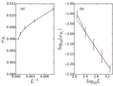
0.000 0.003 0.006
Figure 6: (a) Stochastic lattice simulation of the two-predator-one-prey model with
‘Dar-winian’ evolution only introduced to the predation efficienciesη: critical distribution width
ωBcas a function of the inverse linear system size 1/L, with predator death rateµ= 0.125,
prey reproduction rateσ = 1.0, and ωηA = 0.1. The data are obtained for linear system
sizesL∈[128,256,512,1024,2048]. (b) Double-logarithmic plot of the critical widthωBcas a
function of system sizeL; the red straight line represents a simple linear regression of the four points withL∈[256,512,1024,2048], with slope−0.2. The point withL= 128 presumably deviates from this straight line due to additional strong finite-size effects.
predator species was 50%. With the simulations on a 512×512 system and
all the parameters set as mentioned above, ωBc was measured to be close to
0.008. We repeated these measurements for various linear system sizes L in
the range [128,2048]. Fig. 6(a) shows ωBc as a function of 1/L, indicating
that ωBc decreases with a divergent rate as the system is enlarged. Because
of limited computational resources, we were unable to extend these results to
even larger systems. According to the double-logarithmic analysis shown in
Fig. 6(b), we presume thatωBcwould fit a power lawωBc∼L−θwith exponent
θ = 0.2. This analysis suggests that ωBc = 0 in an infinitely large system,
and that the reentrant transition from B survival to A survival in the range
ωηB∈[0, ωηA] is likely a finite-size effect. We furthermore conclude that in the
three-species system (two predators and a single prey) the predator species with
one. A smaller ω means that the offspring’s efficiency is more centralized at
its parent’s efficacy; mutations and adaptations have smaller effects. Evolution
may thus optimize the overall population efficiency to higher values and render
this predator species stronger than the other one with largerω, which is subject
to more, probably deleterious, mutations. These results were all obtained from
the measurements withωηA= 0.1. However, other values of ωηAincluding 0.2,
0.3, and 0.4 were tested as well, and similar results observed.
Our numerical observation that two predator species cannot coexist
contra-dicts observations in real ecological systems. This raises the challenge to explain
multi-predator-species coexistence. Notice that ‘Darwinian’ evolution was only
applied to the predation efficiency in our model. However, natural selection
could also cause lower predator death rates and increased prey reproduction
rates so that their survival chances would be enhanced in the natural
selec-tion competiselec-tion. One ecological example are island lizards that benefit from
decreased body size because large individuals will attract attacks from their
competitors [5]. In the following, we adjust our model so that the other two
reaction ratesµandσdo not stay fixed anymore, but instead evolve by
follow-ing the same mechanism as previously implemented for the predation efficacies
η. The death rate of an offspring predator particle is hence generated from
a truncated Gaussian distribution centered at its parent’s value, with positive
standard deviationsωµAandωµB for speciesAandB, respectively. The
(trun-cated) Gaussian distribution width for the prey reproduction rate is likewise set
to a non-zero valueωσ.
In the simulations, the initial population densities for all three species are
set at 0.3 with the particles randomly distributed on the lattice. The reaction
rates and efficiencies for these first-generation individuals were chosen asηA0=
ηB0 = ηC0 = 0.5, µA0 =µB0 = 0.125, and σ0 = 1.0. With this same initial
set, we ran simulations with different values of the Gaussian distribution widths
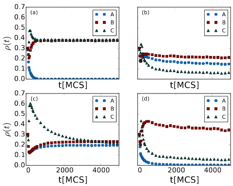
ω. Figure 7 displays the temporal evolution of the three species’ population
densities with four sets of given widthsω: In Fig. 7(a),ωηA= 0.11,ωηB= 0.1,
t[MCS]
Figure 7: Population densitiesρ(t) from Monte Carlo simulations with ‘Darwinian’ evolution introduced to both the predation efficienciesη and predator death rates µ, while the prey reproduction rate stays fixed atσ = 1.0. The species are indicated as blue dots forA, red squares forB, and green triangles for C. The final states are in (a)Aextinction; (b) and (c) transient three-species coexistence; and (d)Bextinction, withωηA = 0.11,ωµA = 0.3,
ωµB = 0.125 in (a),ωηA = 0.08, ωµA = 0.1,ωµB = 0.09 in (b), ωηA = 0.08, ωµA= 0.4,
ωµB = 0.39 in (c), and ωηA = 0.08, ωµA = 0.4, ωµB = 0.09 in (d), while ωηB = 0.1,
ω gives advantages to the corresponding species, ωηB < ωηA and ωµB < ωµA
render predators B stronger than A in general. As the graph shows, species
Adies out quickly and finally only B and C remain in the system. In all four
cases, the preyCstay active and do not become extinct.
However, it is not common that a species is stronger than others in every
aspect, so we next setωso thatAhas advantages overBin predation, i.e.,ωηA<
ωηB, but is disadvantaged through broader-distributed death ratesωµA> ωµB.
In Fig. 7(b), ωηA = 0.08, ωηB = 0.1, ωηC = 0.1, ωµA = 0.1, ωµB = 0.09,
and ωσC = 0; in Fig. 7(c), ωηA = 0.08, ωηB = 0.1, ωηC = 0.1, ωµA = 0.4,
ωµB = 0.39, and ωσC = 0. In either case, none of the three species becomes
extinct after 10 000 MCS, and three-species coexistence will persist at least for
much longer time. Monitoring the system’s activity, we see that the system
remains in a dynamic state with a large amount of reactions happening. When
we repeat the measurements with other independent runs, similar results are
observed, and we find the slow decay of the population densities to be rather
insensitive to the specific values of the widthsω. As long as we implement a
smaller width ω for the A predation efficiency than for the B species, but a
larger one for its death rates, or vice versa, three-species coexistence emerges.
Of course, when the values of the standard deviationsωdiffer too much between
the two predator species, one of them may still approach extinction fast. One
example is shown in Fig. 7(d), where ωηA = 0.08, ωηB = 0.1, ωηC = 0.1,
ωµA= 0.4,ωµB= 0.09, andωσC = 0; sinceωµA is about five times larger than
ωµB here, the predation advantage of species A cannot balance its death rate
disadvantage, and consequently speciesAis driven to extinction quickly. Yet the
coexistence of all three competing species in Figs. 7(b) and (c) does not persist
forever, and at least one species will die out eventually, after an extremely long
time. Within an intermediate time period, which still amounts to thousands
of generations, they can be regarded as quasi-stable because the decay is very
slow. This may support the idea that in real ecosystems perhaps no truly stable
multiple-species coexistence exists, and instead the competing species are in fact
In Figs. 7(a) and (d), the predatorA population densities decay exponentially
with relaxation times of order 100 MCS, while the corresponding curves in (b)
and (c) approximately follow algebraic functions (power law decay).
However, we note that in the above model implementation the range of
predator death ratesµ was the entire interval [0,1], which gives some
individ-uals a very low chance to decay. Hence these particles will stay in the system
for a long time, which accounts for the long-lived transient two-predator
coex-istence regime. To verify this assumption, we set a positive lower bound on
the predators’ death rates, preventing the presence of near-immortal
individu-als. We chose the value of the lower bound to be 0.001, with the death rates
µfor either predator species generated in the predation and reproduction
pro-cesses having to exceed this value. Indeed, we observed no stable three-species
coexistence state, i.e., one of the predator species was invariably driven to
ex-tinction, independent of the values of the widths ω, provided they were not
exactly the same for the two predator species. To conclude, upon introducing
a lower bound for their death rates, the two predator species cannot coexist
despite their dynamical evolutionary optimization.
4. Effects of direct competition between both predator species
4.1. Inclusion of direct predator competition and mean-field analysis
We proceed to include explicit direct competition between both predator
species in our model. The efficiencies of predator particles are most likely to
be different since they are randomly generated from truncated Gaussian
distri-butions. When a strong A individual (i.e., with a large predation efficacy η)
meets a weakerB particle on an adjacent lattice site, or vice versa, we now
al-low predation between both predators to occur. Direct competition is common
within predator species in nature. For example, a strong lizard may attack and
even kill a small lizard to occupy its habitat. A lion may kill a wolf, but an
adult wolf might kill an infant lion. Even though cannibalism occurs in nature
differ-ent predator species. In our model, direct competition between the predator
species is implemented as follows: For a pair of predatorsAi andBj located on
neighboring lattice sites and endowed with respective predation efficienciesηAi
andηBj < ηAi, particleBj is replaced by a newAparticleAz with probability
ηAi−ηBj; conversely, ifηAi< ηBj, there is a probability ηBj −ηAi that Ai is
replaced by a new particleBz.
We first write down and analyze the mean-field rate equations for the
sim-pler case when the predator species compete directly without evolution, i.e.,
all reaction rates are uniform and constant. We assume thatA is the stronger
predator with λA > λB, hence only the reaction A+B → A+A is allowed
to take place with rate λA−λB, but not its complement, supplementing the
original reaction scheme listed in (1). The associated mean-field rate equations
read
with the non-zero stationary solutions
(i) a= 0, b= σ(KλB−µB)
Within this mean-field theory, three-species coexistence states exist only when
the total initial population density is set toa(0) +b(0) +c(0) =µA−µB
λA−λB. In our
lattice simulations, however, we could not observe any three-species coexistence
state even when we carefully tuned one reaction rate with all others held fixed.
Next we reinstate ‘Darwinian’ evolution for this extended model with direct
competition between the predator species. We utilize the function ˆλij =|ηi−ηj|
predator death rate µ is fixed for both species A and B, the ensuing
quasi-Since a closed set of solutions for eqs. (9) is very difficult to obtain, we resort
to numerical integration. As before, we rely on an explicit fourth-order Runge–
Kutta scheme with time step ∆t= 0.1, initial conditionsai(t= 0) =bi(t= 0) =
ci(t= 0) = 1/N, number of subspeciesN = 100, and carrying capacity K= 3.
Four examples for such numerical solutions of the quasi-subspecies mean-field
equations are shown in Fig. 8, and will be discussed in the following subsection.
4.2. The quasi-stable three-species coexistence region
For the three-species system with two predators A,B and preyC, we now
introduce ‘Darwinian’ evolution to both the predator death rates µ and the
predation efficienciesη. In addition, we implement direct competition between
the predatorsAand B. We set the lower bound of the death ratesµto 0.001
for both predator species. The simulations are performed on a 512×512 square
lattice with periodic boundary conditions. Initially, individuals from all three
species are randomly distributed in the system with equal densities 0.3. Their
initial efficiencies are chosen as ηA = 0.5 = ηB and ηC = 0. Since there is no
evolution of the prey efficiency, ηC will stay zero throughout the simulation.
100 101 102 103
Figure 8: Numerical solutions of the mean-field equations (9) for the two-predator subspecies
densitiesa(t) = 1
ibi(t) (solid) for different distribution
widthsωη,B and the parametersωη,A= 0.14,ωη,C=∞,σ= 1, andµ= 0.5. (a) Population
densities in the presence of direct predator-predator competition; and (b) in the absence of
this competition. Note that three-species coexistence is only possible when direct
predator-predator competition is explicitly implemented.
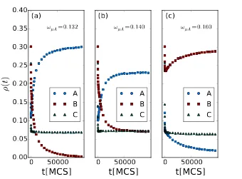
and ωηB = 0.15, giving species A an advantage over B in the non-linear
pre-dation process. We select the width of the death rate distribution of species
B as ωµB = 0.1. If ωµA is also chosen to be 0.1, the B population density
would decay exponentially. ωµA> ωµB = 0.1 is required to balance speciesA’s
predation adaptation advantage so that stable coexistence is possible. Figure 9
shows the population densities resulting from our individual-based Monte Carlo
simulations as a function of time, for different valuesωµA = 0.132, 0.140, and
0.160. These graphs indicate the existence of phase transitions from speciesB
extinction in Fig. 9(a) to predatorA-Bcoexistence in Fig. 9(b), and finally toA
extinction in Fig. 9(c)). In Fig. 9(a), speciesAis on average more efficient than
B in predation, but has higher death rates. Predator species B is in general
the weaker one, and hence goes extinct after about 100 000 MCS. Figure 9(b)
shows a (quasi-)stable coexistence state with neither predator species dying out
within our simulation time. In Fig. 9(c),ωµA is set so high thatAparticles die
much faster thanB individuals, so that finally species Awould vanish entirely.
0 50000
Figure 9: Data obtained from Monte Carlo simulations where both direct competition between
both predator species as well as evolutionary dynamics are introduced: Temporal population
density record withωηA = 0.1, ωηB = 0.15, ωµB = 0.1 andωµA = 0.132, 0.140, 0.160
(from left to right) with speciesAindicated with blue dots,Bred-dashed, andC with green triangles.
quasi-subspecies mean-field model (9) for four different values of the speciesB
efficiency widthωη,B. In particular, it shows that there is a region of coexistence
in which both predator species reach a finite steady-state density, supporting the
Monte Carlo results from the stochastic lattice model. In contrast, numerical
solutions of eqs. (9) with ˆλij = 0, equivalent to eqs. (3), exhibit no three-species
coexistence region; see Fig. 8(b).
At an active-to-absorbing phase transition threshold, one should anticipate
the standard critical dynamics phenomenology for a continuous phase
transi-tion: exponential relaxation with time becomes replaced by much slower
0 5000 10000
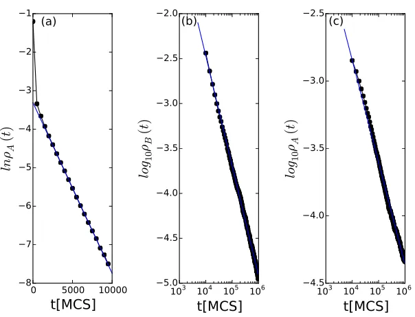
Figure 10: Monte Carlo simulations with direct predator competition: (a) Exponential decay
of the predator population density ρA(t) with ωµA = 0.2, ωηA = 0.1, ωηB = 0.15, and
ωµB = 0.1; the blue straight line is obtained from a linear regression of the data points
forx≥2000, with slope−0.00044. (b) Algebraic power-law decay of the predatorBspecies density withωµA= 0.136 and the other parameters set as in (a). (c) Power-law decay ofρA(t)
forωµA= 0.159. The black dots are measured population densities from the simulations, while
the blue straight lines indicate simple linear regressions of the simulation data.
coexistence range for our otherwise fixed parameter set to be in the range
ωµA ∈ [0.136,0.159]. Figure 10(a) shows an exponential decay of the
preda-tor population A density with ωµA = 0.2, deep in the absorbing extinction
phase. The system would attainB-C two-species coexistence within of the
or-der 104 MCS. We also ran the Monte Carlo simulation with ω
µA = 0.1, also
inside an absorbing region, but now with speciesBgoing extinct, and observed
exponential decay of ρB(t). By changing the value of ωµA to 0.136 as
plot-ted in Fig. 10(b), ρB(t)∼ t−αB fits a power law decay with critical exponent
αB = 1.22. Since it would take infinite time forρB to reach zero while species
0 2 4 6 8 10 12 14
Figure 11: Monte Carlo simulations with direct predator competition. Main panel:
Quasi-stationary correlation functionsC(x) after the system has evolved for 10 000 MCS withωµA=
0.147,ωηA = 0.1,ωηB = 0.15, andωµB = 0.1, when the system resides in the coexistence
state. Inset: temporal evolution of the correlation lengthξ(t); all lengths are measured in units of the square lattice spacing.
at this point already resides at the threshold of three-species coexistence. Upon
increasingωµA further, all three species densities would reach their asymptotic
constant steady-state values within a finite time and then remain essentially
constant (with small statistical fluctuations). At the other boundary of this
three-species coexistence region, ωµA = 0.159, the decay of ρA(t) also fits a
power law as depicted in Fig. 10(c), and ρB(t) would asymptotically reach a
positive value. However, the critical power law exponent is in this case
es-timated to be αA = 0.76. We do not currently have an explanation for the
distinct values observed for the decay exponentsαA and αB, neither of which
are in fact close to the corresponding directed-percolation valueα= 0.45 [41].
If we increaseωµA even more, speciesAwould die out quickly and the system
subsequently reduce to aB-C two-species predator-prey coexistence state. We
remark that the critical slowing-down of the population density at either of the
two thresholds as well as the associated critical aging scaling may serve as a
It is of interest to study the spatial properties of the particle distribution.
We choose ωµA = 0.147 so that the system resides deep in the three-species
coexistence region according to Fig. 10. The correlation functions are
mea-sured after the system has evolved for 10 000 MCS as shown in the main plot
of Fig. 11. The results are similar to those in the previous sections in the sense
that particles are positively correlated with the ones from the same species, but
anti-correlated to individuals from other species. The correlation functions for
both predator species are very similar: CAA(x) andCBB(x) overlap each other
forx≥5, andCAC andCBC coincide forx≥2 lattice sites. The inset displays
the measured characteristic correlation length as functions of simulation time,
each of which varies on the scale of ∼0.1 during 70 000 MCS, indicating that
the species clusters maintain nearly constant sizes and keep their respective
dis-tances almost unchanged throughout the simulations. The correlation lengths
ξAA andξBBare very close and differ only by less than 0.2 lattice sites. These
data help to us to visualize the spatial distribution of the predators: The
indi-viduals of bothAandBspecies arrange themselves in clusters with very similar
sizes throughout the simulation, and their distances to prey clusters are almost
the same as well. Hence predator speciesAandB are almost indistinguishable
in their spatial distribution.
4.3. Monte Carlo simulation results in a zero-dimensional system
The above simulations were performed on a two-dimensional system by
lo-cating the particles on the sites of a square lattice. Randomly picked particles
are allowed to react (predation, reproduction) with their nearest neighbors.
Spatial as well as temporal correlations are thus incorporated in the reaction
processes. In this subsection, we wish to compare our results with a system
for which spatial correlations are absent, yet which still displays manifest
tem-poral correlations. To simulate this situation, we remove the nearest-neighbor
restriction and instead posit all particles in a ‘zero-dimensional’ space. In the
resulting ‘urn’ model, the simulation algorithm entails to randomly pick two
individ-0 50000
t[MCS]
0.00 0.05 0.10 0.15 0.20 0.25 0.30 0.35 0.40
ρ(
t)
(a)
A B C
0 50000
t[MCS]
(b)
A B C
0 50000
t[MCS]
(c)
A B C
Figure 12: Data obtained from single Monte Carlo simulation runs in a zero-dimensional
system with direct competition and evolutionary dynamics, hence only temporal but no spatial
correlations: Time record of the population densities for all three species withωηA = 0.1,
ωηB = 0.15, ωµB = 0.1 and ωµA = 0.132,0.140,0.160 (from left to right), with species A
indicated with blue dots,Bred-dashed, andCwith green triangles.
ual character values. We find that if all the particles from a single species are
endowed with homogeneous properties, i.e., the reaction rates are fixed and
uniform as in section 2, no three-species coexistence state is ever observed. If
evolution is added without direct competition between predator species as in
section 3, the coexistence state does not exist neither. Our observation is again
that coexistence occurs only when both evolution and direct competition are
introduced. Qualitatively, therefore, we obtain the same scenarios as in the
two-dimensional spatially extended system. The zero-dimensional system
how-ever turns out even more robust than the one on a two-dimensional lattice, in
in parameter space. Figure 12 displays a series of population density time
evo-lutions from single zero-dimensional simulation runs with identical parameters
as in Fig. 9. All graphs in Fig. 12 reside deeply in the three-species coexistence
region, while Fig. 9(a) and (c) showed approaches to absorbing states with one
of the predator species becoming extinct. With ωηA = 0.1, ωηB = 0.15, and
ωµB = 0.1 fixed, three-species coexistence states in the zero-dimensional system
are found in the region ωµA ∈(0,1), which is to be compared with the much
narrower interval (0.136,0.159) in the two-dimensional system, indicating that
spatial extent tends to destabilize these systems.
This finding is in remarkable contrast to some already well-studied systems
such as the three-species cyclic competition model, wherein spatial extension
and disorder crucially help to stabilize the system [43, 44]. Even though we do
not allow explicit nearest-neighbor ‘hopping’ of particles in the lattice simulation
algorithm, there still emerges effective diffusion of prey particles followed by
predators. Since predator individuals only have access to adjacent prey in the
lattice model, the presence of one predator species would block their neighboring
predators from their prey. Imagining a cluster of predator particles surrounded
by the other predator species, they will be prevented from reaching their ‘food’
and consequently gradually die out. However, this phenomenon cannot occur
in the zero-dimensional system where no spatial structure exists at all, and
hence blockage is absent. In the previous section we already observed that
the cluster size of predator species remains almost unchanged throughout the
simulation process when the total population size of the weaker predator species
gradually decreases to zero, indicating that clusters vanish in a sequential way.
We also noticed that population densities reach their quasi-stationary values
much faster in the non-spatial model, see Fig. 12, than on the two-dimensional
lattice, Fig. 9. In the spatially extended system, particles form intra-species
clusters, and reactions mainly occur at the boundaries between neighboring such
clusters of distinct species, thus effectively reducing the total reaction speed.
This limiting effect is absent in the zero-dimension model where all particles
0.000 0.005 0.010
Figure 13: Monte Carlo simulations with direct predator competition: The final distribution
of predation efficienciesη and predator death rates µafter the system has stabilized after 50 000 MCS with initial distribution widthsωηA = 0.15,ωηB = 0.1,ωµB = 0.1 andωµA ∈
[0.144,0.15,0.156]; data indicated respectively with red squares, blue triangles up, and green triangles down. (a) and (c) depict the distribution of characters of predator speciesA, while (b) and (d) that ofB. The interval [0,1] is divided evenly into 1 000 histogram bins; the quantityP represents the proportion of individuals with rates in the corresponding bins.
4.4. Character displacements
Biologists rely on direct observation of animals’ characters such as beak size
when studying trait displacement or evolution [6, 2, 7, 8, 32, 33, 34, 35].
Inter-specific competition and natural selection induces noticeable character changes
within tens of generations so that the animals may alter their phenotype, and
thus look different to their ancestors. On isolated islands, native lizards change
the habitat use and move to elevated perches following invasion by a second
lizard kind with larger body size. In response, the native subspecies may evolve
bigger toepads [45]. When small lizards cannot compete against the larger ones,
character displacement aids them to exploit new living habitats by means of
de-veloping larger toepads in this case, as a result of natural selection.
preda-tion efficiencies η and death rates µ are allowed to be evolving features of the
individuals. In Fig. 13, the predation efficiency η is initially uniformly set to
0.5 for all particles, and the death rate µ = 0.5 for all predators (of either
species). Subsequently, in the course of the simulations the values of any
off-spring’sη and µ are selected from a truncated Gaussian distribution centered
at their parents’ characters with distribution widthωη andωµ. When the
sys-tem arrives at a final steady state, the values ofη andµ too reach stationary
distributions that are independent of the initial conditions. We already
demon-strated above that smaller widthsω afford the corresponding predator species
advantages over the other, as revealed by a larger and stable population
den-sity. In Fig. 13, we fixωηA= 0.15,ωηB= 0.1,ωµB= 0.1, and choose values for
ωµA ∈ [0.144,0.15,0.156] (represented respectively by red squares, blue
trian-gles up, and green triantrian-gles down), and measure the final distribution ofη and
µwhen the system reaches stationarity after 50 000 MCS. Figures 13(a) and (c)
show the resulting distributions for predator speciesA, while (b) and (d) those
forB. Since bothµandη are in the range [0,1], we divide this interval evenly
into 1 000 bins, each of length 0.001. The distribution frequencyP is defined
as the number of individuals whose character values fall in each of these bins,
divided by the total particle number of that species. In Fig. 13(a), the eventual
distribution ofµA is seen to become slightly less optimized asωµA is increased
from 0.144 to 0.156 since there is a lower fraction of lowµAvalues in the green
curve as compared with the red one. Since speciesAhas a larger death rate, its
final stable population density decreases asµAincreases. In parallel, the
distri-bution ofηA becomes optimized as shown in Fig. 13(c), as a result of natural
selection: SpeciesA has to become more efficient in predation to make up for
its disadvantages associated with its higher death rates. Predator speciesB is
also influenced by the changes in species A. Since there is reduced
competi-tion fromAin the sense that its population number decreases, theB predators
gain access to more resources, thus lending its individuals with low predation
efficiencies better chances to reproduce, and consequently rendering the
0 20 40 60 80 100 120
0 1000 2000 3000 4000 5000
t[MCS]
Figure 14: Monte Carlo simulations showing the temporal record of both predator
popula-tion densities when the distribupopula-tion widthsωηA andωηB periodically exchange their values
between 0.2 and 0.3. The other parameters are set to µA = µB = 0.125,σ = 1.0, and
ωC=ωµA=ωµB= 0. The switch periods areT = 10 MCS in (a) andT = 400 MCS in (b).
as predator speciesB needs no longer become as efficient in predation because
they enjoy more abundant food supply. In that situation, since speciesB does
not perform as well as before in predation, their death rateµB distribution in
turn tends to become better optimized towards smaller values, as is evident in
Fig. 13(b).
4.5. Periodic environmental changes
Environmental factors also play an important role in population abundance.
There already exist detailed computational studies of the influence of spatial
variability on the two-species lattice LV model [43, 31, 37]. However, rainfall,
temperature, and other weather conditions that change in time greatly
deter-mine the amount of food supply. A specific environmental condition may favor
one species but not others. For example, individuals with larger body sizes
various characters favoring certain natural conditions, one may expect
environ-mental changes to be beneficial for advancing biodiversity.
We here assume a two-predator system with speciesA stronger than B so
that the predatorB population will gradually decrease as discussed in section
3. Yet if the environment changes and turns favorable to species B before it
goes extinct, it may be protected from extinction. According to thirty years of
observation of two competing finch species on an isolated island ecology [32],
there were several instances when environmental changes saved one or both of
them when they faced acute danger of extinction. We takeωηAandωηBas the
sole control parameters determining the final states of the system, holding all
other rates fixed in our model simulations. Even though the environmental
fac-tors cannot be simulated directly here, we may effectively address
environment-related population oscillations by changing the predation efficiency distribution
widthsω. We initially setωηA= 0.2 andωηB= 0.3, with the other parameters
held constant atµA=µB = 0.125,σ= 1.0, andωC =ωµA=ωµB = 0. In real
situations the environment may alternate stochastically; in our idealized
sce-nario, we just exchange the values ofωηAandωηB periodically for the purpose
of simplicity. The population average of the spontaneous death rate is around
0.02, therefore its inverse ≈50 MCS yields a rough approximation for the
in-dividuals’ typical dwell time on the lattice. When the time period T for the
periodic switches is chosen as 10 MCS, which is shorter than one generation’s
life time, the population densities remain very close to their identical mean
values, with small oscillations; see Fig. 14(a). Naturally, neither species faces
the danger of extinction when the environmental change frequency is high. In
Fig. 14(b), we study the case of a long switching timeT = 400 MCS, or about
eight generations. As one would expect, theB population abundance decreases
quickly within the first period. Before the B predators reach total extinction,
the environment changes to in turn rescue this speciesB. This example shows
that when the environment stays unaltered for a very long time, the weaker
species that cannot effectively adapt to this environment would eventually
periodT close matches the characteristic decay timetc, see Fig. 14(b), one
ob-serves a resonant amplification effect with large periodic population oscillations
enforced by the external driving.
5. Summary
In this paper, we have used detailed Monte Carlo simulations to study an
ecological system with two predator and one prey species on a two-dimensional
square lattice. The two predator species may be viewed as related families,
in that they pursue the same prey and are subject to similar reactions, which
comprise predation, spontaneous death, and (asexual) reproduction. The most
important feature in this model is that there exists only one mobile and
repro-ducing food resource for all predators to compete for. We have designed different
model variants with the goal of finding the key properties that could stabilize
a three-species coexistence state, and thus facilitate biodiversity in this simple
idealized system. We find no means to obtain such coexistence when all reaction
rates are fixed or individuals from the same species are all homogeneous, which
clearly indicates the importance of demographic variability and evolutionary
population adaptation. When dynamical optimization of the individuals in the
reproduction process is introduced, they may develop various characters related
to their predation and reproduction efficiencies. However, this evolutionary
dy-namics itself cannot stabilize coexistence for all three species, owing to the fixed
constraint that both predator kinds compete for the same food resource. In
our model, direct competition between predator species is required to render
a three-species coexistence state accessible, demonstrating the crucial
impor-tance of combined mutation, competition, and natural selection in stabilizing
biodiversity.
We observe critical slowing-down of the population density decay near the
predator extinction thresholds, which also serves as an indicator to locate the
coexistence region in parameter space. When the system attains its quasi-steady
even as the system evolves further. Character displacements hence occur as a
result of inter-species competition and natural selection in accord with biological
observations and experiments. Through comparison of the coexistence regions
of the full lattice model and its zero-dimensional representation, we find that
spatial extent may in fact reduce the ecosystem’s stability, because the two
predator species can effectively block each other from reaching their prey. We
also study the influence of environmental changes by periodically switching the
rate parameters of the two competing predator species. The system may then
maintain three-species coexistence if the period of the environmental changes is
smaller than the relaxation time of the population density decay. Matching the
switching period to the characteristic decay time can induce resonantly amplified
population oscillations.
Stable coexistence states with all three species surviving with corresponding
constant densities are thus only achieved through introducing both direct
preda-tor competition as well as evolutionary adaptation in our system. In sections 3
and 4, we have explored character displacement without direct competition as
well as competition without character displacement, yet a stable three-species
coexistence state could not be observed in either case. Therefore it is
neces-sary to include both direct competition and character displacement to render
stable coexistence states possible in our model. However, both predator species
AandB can only coexist in a small parameter interval for their predation
effi-ciency distribution widthsω, because they represent quite similar species that
compete for the same resources. In natural ecosystems, of course other factors
such as distinct food resources might also help to achieve stable multi-species
coexistence.
Acknowledgments
The authors are indebted to Yang Cao, Silke Hauf, Michel Pleimling, Per
Rikvold and Royce Zia for insightful discussions. U.D. was supported by a