Epidemic Threshold for the SIRS Model on Networks
M. Ali Saif
Department of Physics
Faculty of Education University of Amran Amran,Yemen
[email protected]
November 20, 2017
Abstract
We study the phase transition from the persistence phase to the extinction phase for the SIRS (susceptible/ infected/ refractory/ susceptible) model of diseases spreading on the net-works. We analytically demonstrate that, in the case when the recovery timeτR is larger than
the infection timeτI, the infection flows on a one direction, i. e. from an infected node to its
susceptible neighbor but, that neighbor can not reinfect that node during its infection time. This behavior leads us to deduce that, when the infection rateλis high enough such that, each infected node on the network infects all its neighbors during its infection time, SIRS model on the network evolves to extinction state, where all nodes on the network become susceptible. Moreover, we assert that, existing the loops on the network are necessary in this case in order to, the infection occurs repeatedly within the nodes on the network. In this case, unlike the other models such as SIS model and SIR model, SIRS model will have two critical thresholds separate the persistence phase from extinction phase. That means, for fixed values ofτI and
τR there are two critical points of infection rate λ1 and λ2, epidemic persists in between of
those two points. We also prove that, in between of these points, there is a value ofλin which the system settles down to stable state with highest infected nodes. We confirm these results numerically by a simulation of regular a one dimension system .
1
Introduction
Dynamic propagation of infectious diseases within a mean filed framework or networking frame has been attracted considerable attention recently [1, 2, 3, 4, 5, 6, 7, 10, 11, 12]. Mean field approach for this problem assumes that, populations are not spatially distributed so that they are fully mixed by means an infective individuals are equally likely to spread the disease to any other member of the population or subpopulation to which they belong [1]. With these zero dimensional models it has been possible to establish many important epidemiological results, including the existence of a population threshold values for the spread of disease [3] and the vaccination levels required for eradication [1, 2], and the effect of stochastic fluctuations on the modulation of an epidemic situation [4]. A second approach assumes spatially distribution of population in a lattice such that the variables at each node represent the state of an individual [5, 6, 7, 10, 11, 12]. An epidemiological model has been investigated on many kinds of networks such regular networks [5, 10], small world networks [5, 7, 8], scale-free networks [9, 11] and random networks [13].
In this work, we aim to find the epidemic threshold which separates the persistence phase, where the infection can spread throughout a population, from the extinction phase, where the infection dies out for SIRS model on networks. Epidemic critical threshold has been derived for some models such as, SIR model on random networks [6, 14], SIS model on random networks [15], SIS model on correlated complex networks [16] and the epidemic model described by a birth-death process [17]. For the SIRS model on the regular 2D network, it was observed that, there are two critical thresholds separate the persistence phase from the extinction phase, i. e. for a fixed value of infection timeτI the epidemic will be persistent when infection rateλis between a minimal critical infection rateλ1and a maximal critical infection rateλ2[18]. In this work, we support those results
analytically and numerically for SIRS model on a regular of 1D network.
2
Model Description
The epidemic model on the networks is defined as follows [5, 7, 11]: if we consider a one dimensional lattice of N nodes. Each node connected to its k neighbors. The nodes can exist in one stage of three state, susceptible (S), infected (I) and refractory (R). Susceptible node can pass to the infected state through contagion by an infected one. Infected node pass to the refractory state after an infection time τI. Refractory nodes return to the susceptible state after a recovery time τR. The contagion is possible only during theS phase, and only by aI node. During theRphase, the nodes are immune and do not infect. The system evolves with discrete time steps. Each node in the network is characterized by a time counterτi(t) = 0,1, ..., τI+τR≡τ0, describing its phase in
the cycle of the disease. The epidemiological stateπi of the node (S, I, orR) depends on the phase in the following way:
πi(t) =S ifτi= 0,
πi(t) =I ifτi∈(1, τI),
πi(t) =R ifτi∈(τI+ 1, τ0) (1)
The state of a node in the next step depends on its current phase in the cycle. A susceptible node stays as such, atτ = 0, until it becomes infected. Once infected, it goes (deterministically) over a cycle that lastsτ0 time steps. During the first τI time steps, it is infected and can potentially transmit the disease to a susceptible neighbor. During the lastτRtime steps of the cycle, it remains in stateR, immune and not contagious. After the cycle is complete, it returns to the susceptible state. This model is usually called SIRS model.
3
Model Analysis
In the following, we consider a synchronous update of a system of N nodes on a lattice. Each node is connected to k neighbors. However, for SIRS the infection can spread repeatedly within the nodes on the network, which means the disease can transfer from the infected node (say i) to its neighbors j1, ..., jk, and these neighbors can also reinfect the node i. Here, we derive an
expression of the probability of descendants j1, ..., jk to reinfect their ancestor i. The probability of descendant j1 to reinfect its ancestor i has been calculated for SIS model, this probability is
infects each of its neighbors with probabilityλ. Infected nodes remain as such for τI time steps, after which they become immune forτRtime steps. Hence, the probability T for the infected node
ito infect one of its neighbors during its infection time is [14, 15, 19]:
T= [1−(1−λ)τI
] (2)
When the node i infects one of its neighbors (sayj1), the nodej1 can only reinfect i after i has
became susceptible again. To calculate the probabilityπof the descendantj1to reinfect its ancestor
i, we assume nodeihas been infected forttime steps before infectingj1. Since the infection time is
τI time steps and recovery time isτRtime steps,ineeds for (τI+τR−t) time steps after infectingj1
to become susceptible. Therefore, the total time in whichj1can infectiisτI−(τI+τR−t) =t−τR. Thus, it is clear that, ift≤τR, the nodeiwill reachS state, whereas the nodej1will have reached
Rstate. In this case, it is impossible for the descendantj1to reinfect its ancestori. However when
t > τR, the probability πis given by conditioning ont[19]:
π=
As we have shown above, when the nodeiinfects any one of its neighbors (sayj1) within time which
ist≤τR, the nodej1 will not able to reinfectiduring its infection time. Now, whenτR> τI, the maximum value oftis t=τI, which is less than τR. Thus, for SIRS model and, when τR > τI an infected node can not reinfect its ancestor, which means, infection can flow only on one direction. This result leads us to infer the following two points in which, SIRS model on the networks evolves to absorbing state under the condition of thatτR> τI.
The first point concerns to the effect of the loops inside a network. To clarify this point, we consider a network which is without loops, e. g. tree like network. For simplicity, we assume also the infection starts with a single node placed into a full susceptible nodes on that network. That infected node can infect some of its neighbors, whereas τR > τI, these neighbors can infect also some of their neighbors but, they can not reinfect that node. Therefore, in this case, each link connects two nodes on the network will transmit the infection only on a one direction. That means, the infection will flow from the first infected node through its branches toward the ends of these branches only on a one direction. Thus, SIRS model on such kind of networks will evolve to absorbing state where, all nodes become susceptible, that will happen for any values of infection time and infection rate. We conclude that, existing the loops on the network are necessary in order to the infection spreads repeatedly within the nodes on the network.
The second point relates to the effect of the values of the parametersτI and λ. To show that effect, let’s suppose the node j1 and node j2 are neighbors, which they have been infected at
preceding timet1andt2respectively. The probability for the nodej1to infectj2will be zero unless
t=t1−t2 is greater thanτR. In general, we define the time delay tfor any connected two nodesi
andj, as follows
Whereti is the time at which the nodeihas been infected, tj is the time at which the node j has been infected. We also define the difference between the infection time and recovery time ∆τ as follows:
∆τ =τR−τI (5)
Now, let’s consider the extremist case, in which each infected node on the network, infects all of its neighbors during its first infection period. If the infection starts at the node i, then, that node will infect all of its neighborsj1, ..., jk during its infection time. Whereas,τR> τI, the nodes
j1, ..., jk will not able to reinfect the node iduring their infection time. Consecutively, the nodes
j1, ..., jk will infect their neighbors but these neighbors also can not reinfect these nodes. Moreover, where the maximum value of t for any two connected neighbors will not exceed the value of τI, which means they can not infect each other. Hence, the infection will propagate away from the center of infection (first infected node) toward the network boundaries, only on a one direction. This means each node on the network will infect only once. Therefore, this system will evolve to disease-free equilibrium in which all nodes become susceptible. Generally, we can say that, for SIRS model on the networks, whenτR > τI, if each infectious node on the network, infects all of
its neighbors during its first stage of infection, SIRS will evolve to an absorbing state where all the nodes on the network become susceptible.We speculate that, such behavior will be correct for SIRS model on any kind of networks.
Here is a question arise, for this model on the networks, how the infection can spread repeatedly within the nodes on the networks? The answer is that, firstly, the network must be contain loops. Secondly, there must be some neighbors on the network which they have been infected at different times, and that difference in time must be greater thanτR. To that happen, it is necessary for some infected nodes on the network, to do not infect all of their neighbors during their infection time. These uninfected nodes, must be infected by another infected neighbor at later time. In this case, we may get some neighbors on the network witht > τR. These neighbors witht > τR, will induce the second period of infection. It is clear here that, the reinfection will happen through the loop of nodes. Hence, the values of τI and λwill play a crucial role for SIRS model on the networks. However, that does not mean the value ofτR has no effect, it is manifest that, for a fixed value of
τI, the possibility of getting a pair of neighbors witht > τRincreases as the value of ∆τ decreases, i. e. when the value of ∆τ is minimum, there is a better chance to get some neighbors on the network witht > τR.
It is clear from the Eq. (2) that, the probability for an infected node to infect its neighbors increases as the infection time or the infection rate increases. An infected node infects more numbers of its neighbors during its infection time as the value ofλor τI becomes bigger. Therefore, there must be a minimum value ofτI as the value ofλis kept fixed, at which each infected node can infect all of its neighbors during its first infection period. Similarly, if we fixτI and increaseλ, there must be a minimum value ofλat which each infected node can infect all of its neighbors during its first infection period. Thus, there is an upper critical threshold which separates the persistence phase from the extinction phase for SIRS model on networks. With Eq. (2) we can find an approximation relation between the infection time and infection probability at which the critical threshold exists. For small values ofλ, we haveT ≈λτI [14]. Therefore, ifλτI = 1 that means, each infected node will infect all of its neighbors during its first infection period. Such system eventually reaches an extinction state. Therefor, the critical threshold which separates the extinction phase from the persistence phase is
0.000 0.002 0.004 0.006 0.008 0.010 0
1000 2000
III
II
I
1E-3 0.01 100
1000
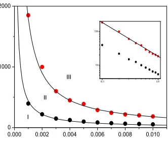
Figure 1: (color on line)Phase diagram of infection time τI as function of infection probability
λ for regular 1D lattice with k = 3 and total population N = 10000. For each point, we set
τR =τI+ 1 and, wait for 10000 time steps. We averaged over 10 independent runs. Inset shows double-logarithmic plot.
However, whenτI <1/λ there is a possibility for SIRS model to settles down to coexistent state with susceptible and infected nodes.
A lower critical threshold we can deduce it from the basic reproductive ratioR0. Which defined
as the average number of secondary infections caused by a single infected node during its infected time when it placed into a full susceptible nodes. Hence, if R0 <1, the introduced infected will
recover without being able to replace themselves by new infections. However, for SIRS model on a network, the expected number of susceptible neighbors that a node has, when it just becomes infected is given byκ−1, where the total expected number of neighbors isκ(whereκ≡
k2
/hki
is the branching factor) [15], and one of them must be excluded as the infected parent from which the current node descended. Then, the mean number of secondary infections per infected node is thus (κ−1)T [15]. The infection will die out if each infected node does not spawn on average at least one replacement so, for a very large network, the critical threshold is given by the relation (κ−1)T = 1 [15]. For small values ofλthe epidemic threshold is:
τI ≡1/(κ−1)λ. (7)
This equation and Eq. (6) show that, the region on the phase space of the parameters (λ,τI) at which the disease will persist, shrinks as the value ofκ−1 decreases. It is clear that, Eq. (7) will collapse on Eq. (6) whenκ= 2. Hence, a persistence phase will not exist whenκ≤2, which is the critical threshold for percolation [15, 19].
In Fig. 1 we plot simulations (dotted curves) and analytical (solid lines) phase diagram for regular 1D system whenk= 3 andN = 10000. Figure shows us clearly the two critical thresholds. The region II corresponding to persistence phase however, the regions I and III corresponding to extinction phases. We fit upper solid curve with the relation τI = aλb where a = 1.85 and
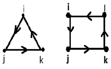
Figure 2: Triangle loop and Square loop.
τI =aλb/(κ−1) whereκ= 6. For best fit, we find that a= 4.2 and b =−0.90±0.01. For this case, the simulation value ofbslightly diverts from the analytical value.
3.2
Case of
τ
R< τ
IFor this case, the total lifetime for disease is greater than recovery time. Therefore, even if each infected node infects all of its neighbors during its infection time, there is still a possibility to get some nodes which has been infected after timet > τR. The probability of these nodes to reinfect their ancestors will be given by Eq. (3). Its clear that, this probability increases as the value of ∆τ
increases. Hence, for this case, the upper critical threshold will not exist.
4
Infection through a loop of nodes
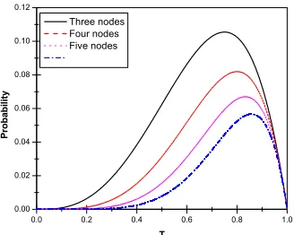
we expected that, where SIRS model has a two critical thresholds then, in between of these critical thresholds there must be a value of λ (for fixed value of τI) at which this system will saturate to stable state with highest infected nodes. To find an approximation relation of that value, we estimate here the probability of occurring the infection through a loop of nodes. We guess that, when the probability of occurring the infection through a loop be maximum, SIRS model will saturate with the maximum infected nodes. Triangles are the smallest loops which linked three nodes. The probability for a node to be infected through a triangle of nodes is:
P =T3(1−T) (8)
Fig.2 shows the triangle and square loop in which (for triangle) the nodeiinfects its neighbor
j with probability T and, does not infect its neighborkwith probability (1-T). The infected node
j now, infects its neighbor kwith probability T, consequently the node k infects the nodei with probability T. Hence, the probability for the nodei to be infected through a triangle of nodes will be given by Eq. 8. This probability has two zero points atT = 0 andT = 1 , it has a peak at
T =3
4 which isλ= 3
(4τI) whenλis small.
The probability for a node to be infected through a square loop of nodes will beT4(1−T). For
a loop of five nodes that probability is T5(1−T) and so on for other loops. In Fig. 3, we plot
0.0 0.2 0.4 0.6 0.8 1.0
Figure 3: Probability of occurring the infection through a loop of nodes as function of T, for different kinds of loops.
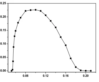
Fig. 4 depicts the steady state of density of infection nodes as function ofλ, for fixed values of
τI = 11 and τR= 12 . Simulations were performed in networks of size up to N = 105, averaging over at least 100 different realizations of the network. As we expected previously system shows pronounced peak at the value ofλ= 0.08±0.01 . This peak coincides approximately with the peak at which the infection through the loops is maximum which is,λ= 0.068 for three nodes,λ= 0.073 for four nodes and λ= 0.076 for five nodes. Figure shows also that, this system has two critical points, upper critical point atλ= 0.21±0.002, whereas lower critical point atλ= 0.052±0.002.
5
Conclusion
0.08 0.12 0.16 0.20 0.00
0.05 0.10 0.15 0.20 0.25
Figure 4: Steady state of density of infection nodes as function of infection probabilityλfor regular 1D network withk= 3, whenτI = 11 andτR= 12.
References
References
[1] Anderson R M and May R M, 1992 Infectious Diseases of Humans: Dynamics and Control
(Oxford: Oxford University Press)
[2] Kermack W O and McKendrick A G,A contribution to the mathematical theory of epidemics, 1927 Proc. R. Soc. Lond. A 115700
[3] Anderson R M and May R M, Vaccination and herd immunity to infectious diseases, 1982 Science 2151053
[4] Landa P and Zaikin A, 1997in Applied Nonlinear Dynamics and Stochastic Systems Near the Millennium, edited by Kadkte J and Bulsara A (AIP, New York, 1997) p.321
[5] Kuperman K and Abramson G, Small world effect in an epidemiological model, 2001 Phys. Rev. Lett. 862909
[6] Pastor-Satorras R and Vespignani A, Epidemic spreading in scale-free networks, 2001 Phys. Rev. Lett. 863200
[7] Gade P M and Sinha S,Dynamic Transitions in Small World Networks: Approach to Equilib-rium, 2005 Phys. Rev. E72052903
[8] da Gama M M T and Nunes A, Epidemics in small world networks, 2006 Eur. Phys. J. B50 205
[10] Roy M and Pascual M,On representing network heterogeneities in the incidence rate of simple epidemic models, 2006 Ecological Comp.380
[11] Yan G, Fu Z Q, Ren J and Wang W X,Collective synchronization induced by epidemic dynamics on complex networks with communities, 2007 Phys. Rev. E75016108
[12] Rozhnova G and Nunes A, Fluctuations and oscillations in a simple epidemic model, 2009 Phys. Rev. E79041922
[13] Liu Z, Lai Y -C and Ye N, Propagation and immunization of infection on general networks with both homogeneous and heterogeneous components, 2003 Phys. Rev. E67031911
[14] Newman M E J,Spread of epidemic disease on networks, 2002 Phys. Rev. E66016128
[15] Parshani R, Carmi S and Havlin S,Epidemic Threshold for the SIS Model on Random Networks, 2010 Phys. Rev. Lett. 104258701
[16] Bogu˜n´a M and Pastor-Satorras R,Epidemic spreading in correlated complex networks, 2002 Phys. Rev. E66047104
[17] Dykman M I, Schwartz I B,and Landsman A S, Disease Extinction in the presence of Random Vaccination, 2008 Phys. Rev. Lett.101078101
[18] Xing Q L, Wang R and Jin Z,Persistence, extinction and spatio-temporal synchronization of SIRS spatial models, 2009 J. Stat. Mech.P07007
[19] Cohen R, Erez K, Avraham D and Havlin S,Resilience of the Internet to Random Breakdowns, 2000 Phys. Rev. Lett. 854626
[20] Watts D J and Strogatz S H,Collective dynamics of small-world networks, 1998 Nature 393 440